A Plot is Worth a Thousand Tests
Assessing Residual Diagnostics with the Lineup Protocol
2024-08-07
🔬 Visual Inference
Suggested by Buja et al. (2009)
🔬 Visual Inference
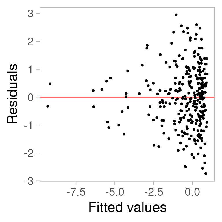
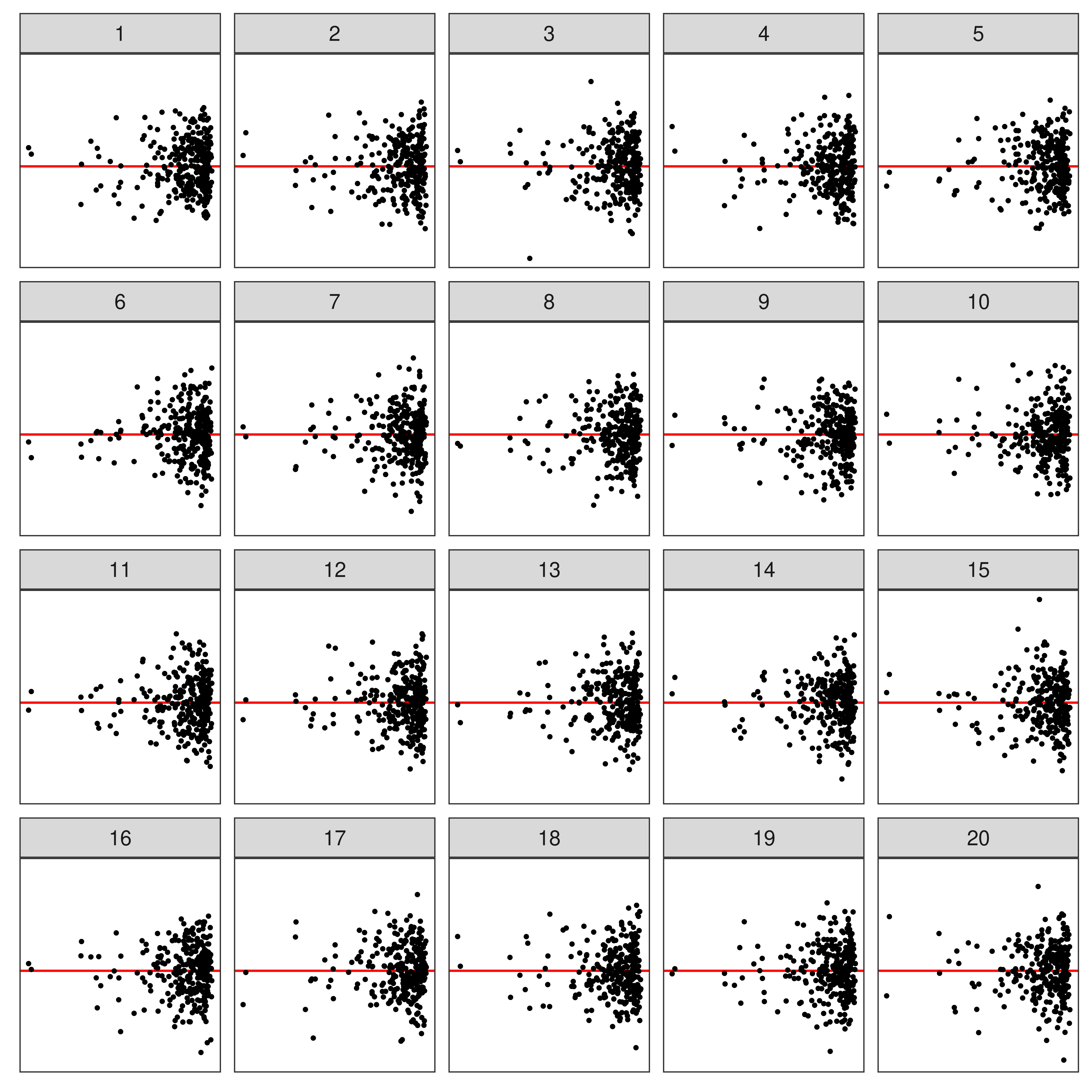
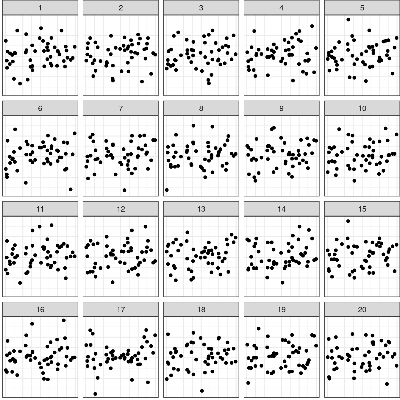
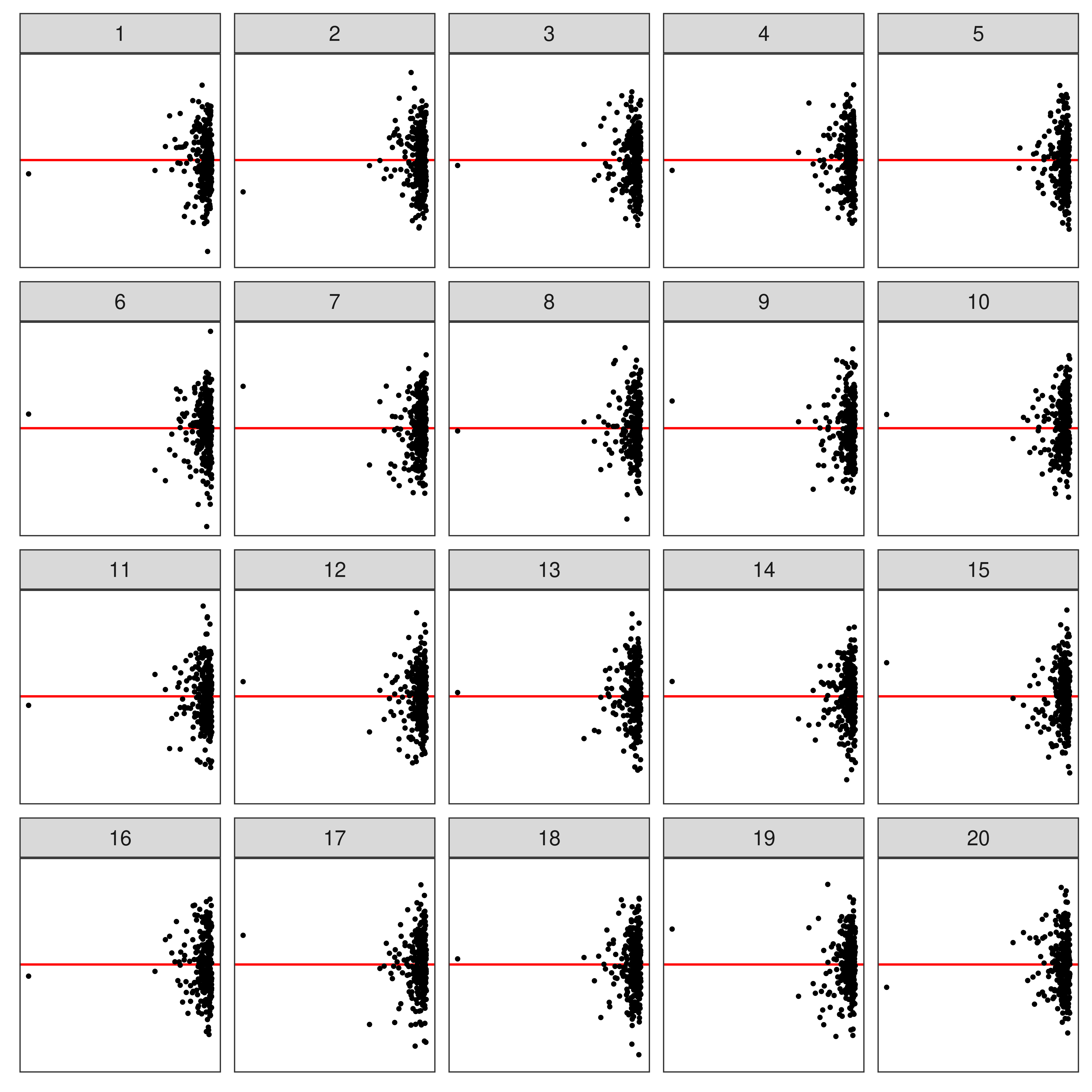
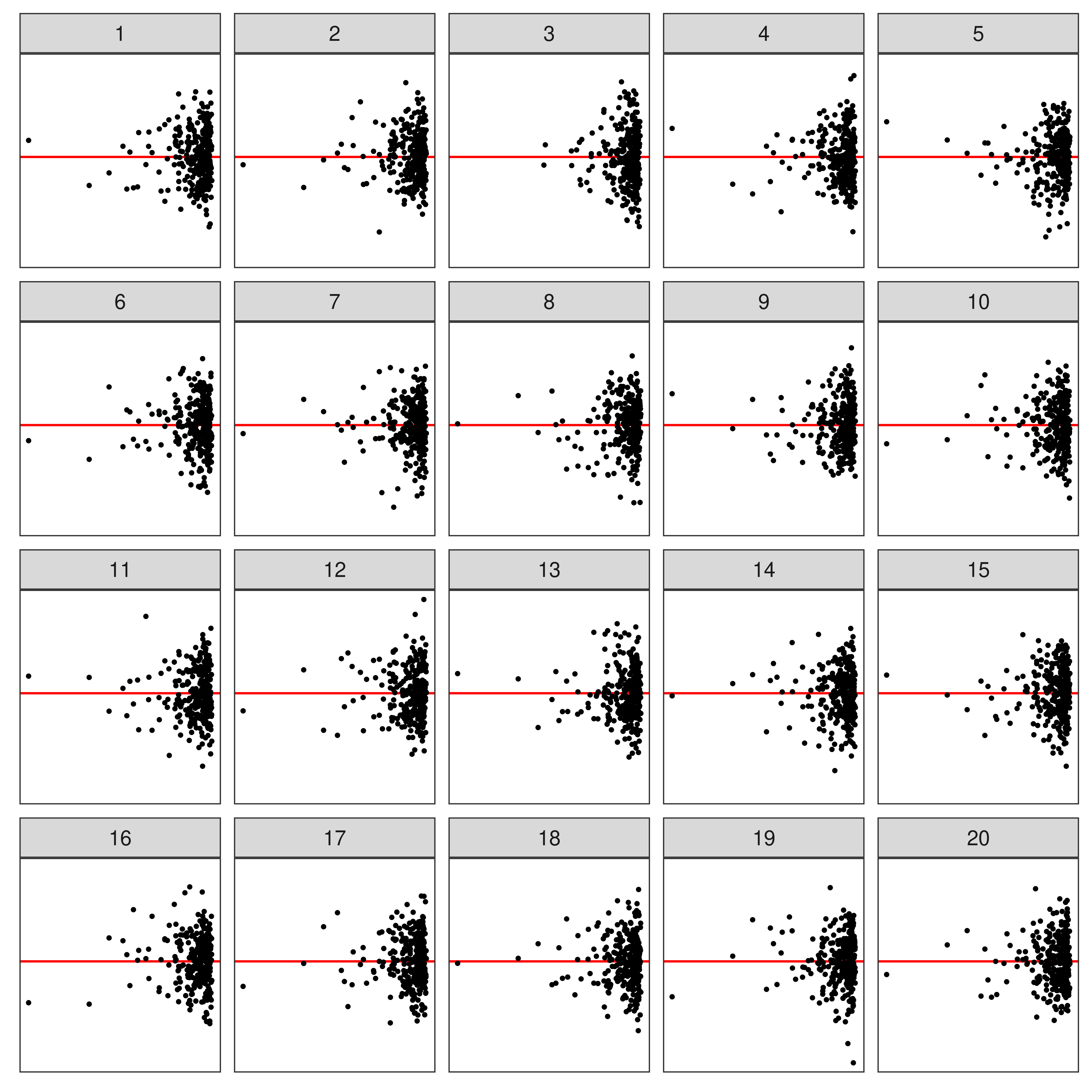
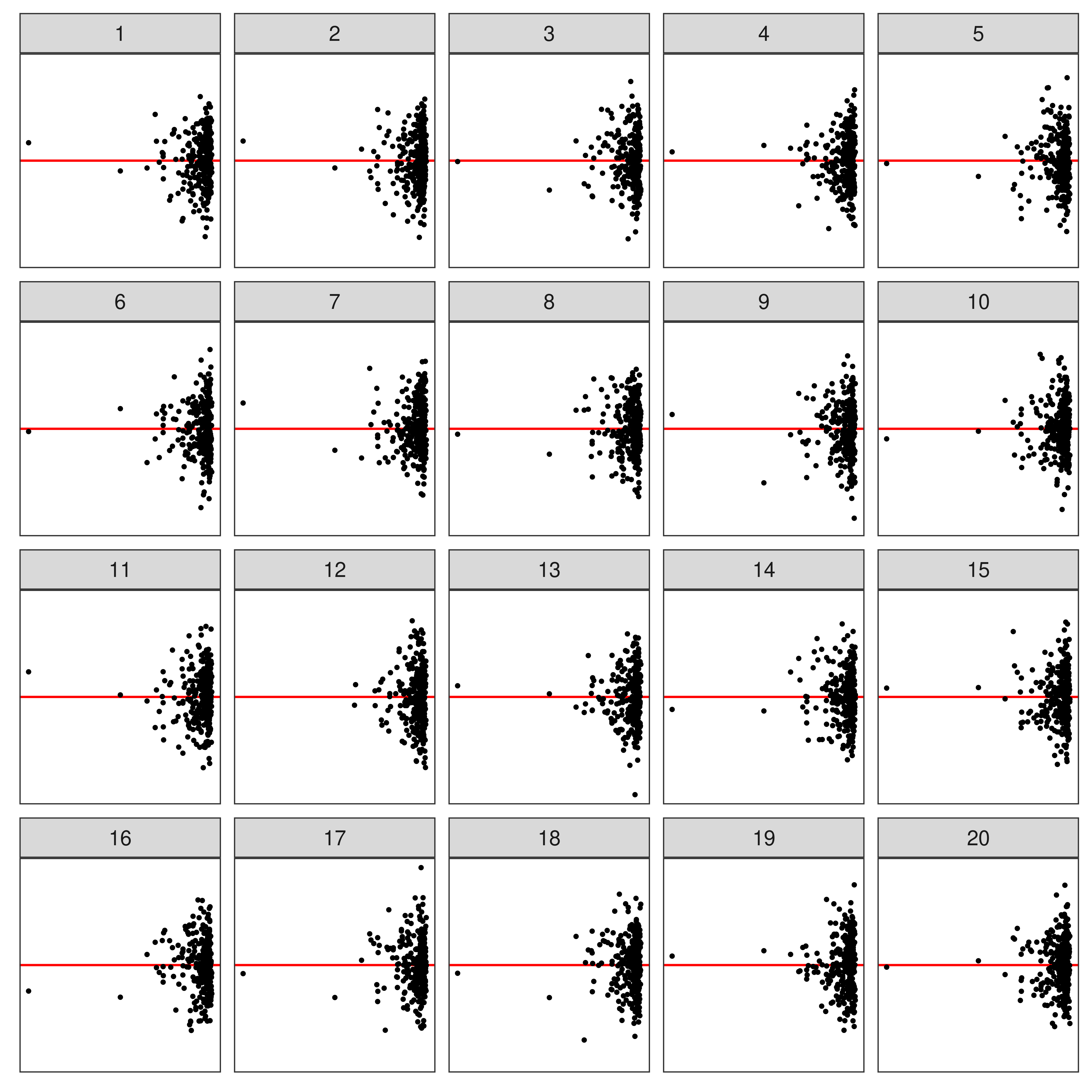
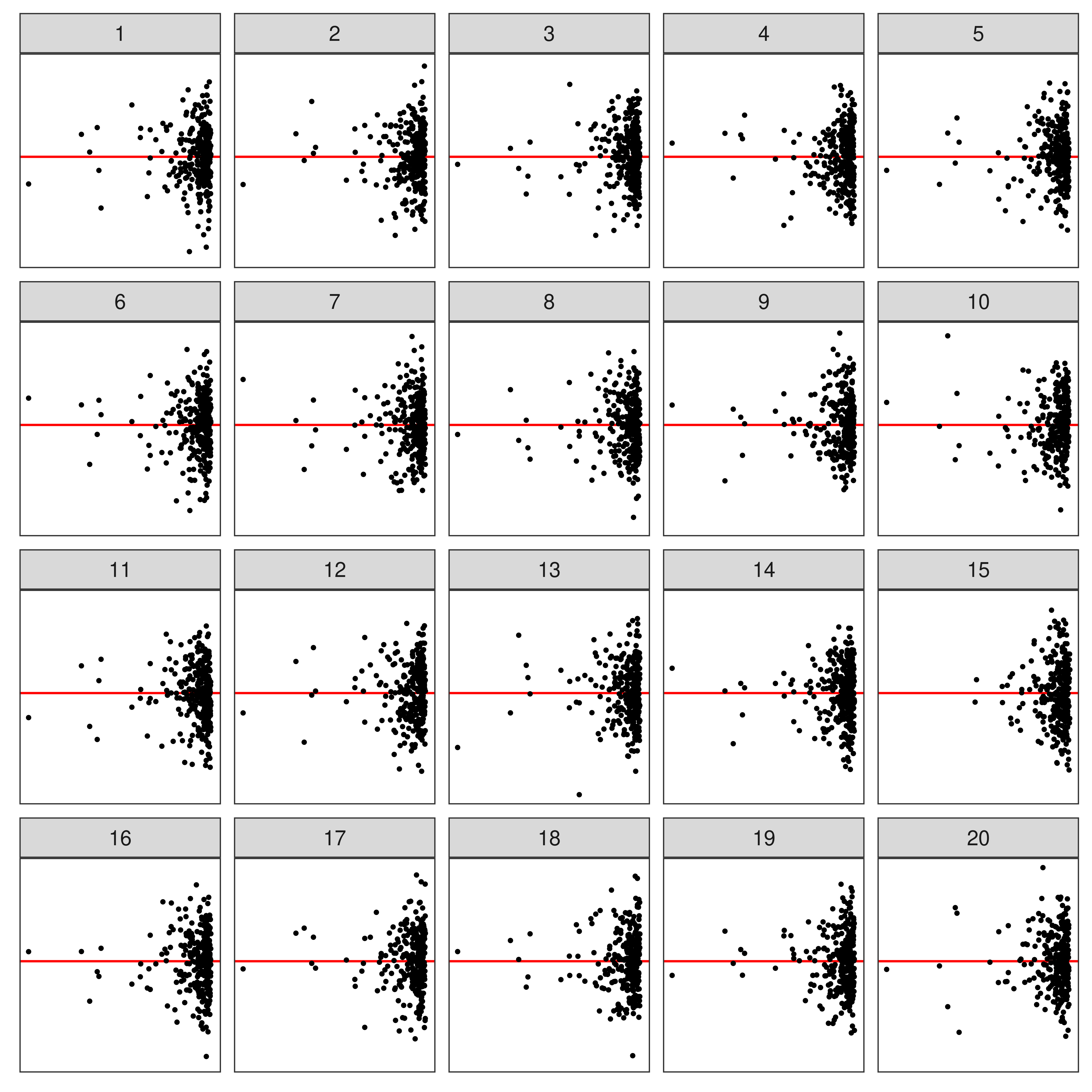
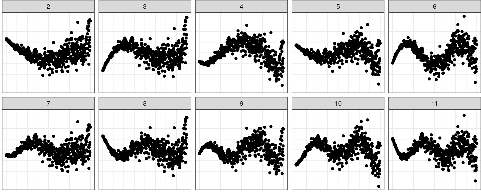
Typically, a lineup of residual plots consists of
- 1 data plot
- 19 null plots w/ residuals simulated from the fitted model.
🔬 Visual Inference
To perform a visual test
- Observer(s) select the most different plot(s).
- P-value (“see value”) can be calculated via a beta-binomial model (VanderPlas et al. 2021)
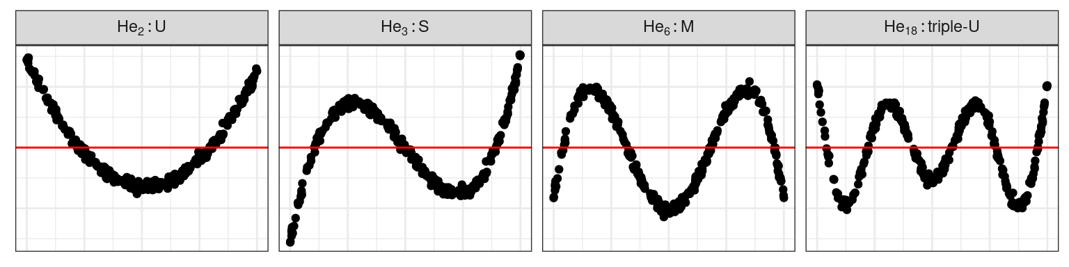
Non-linearity
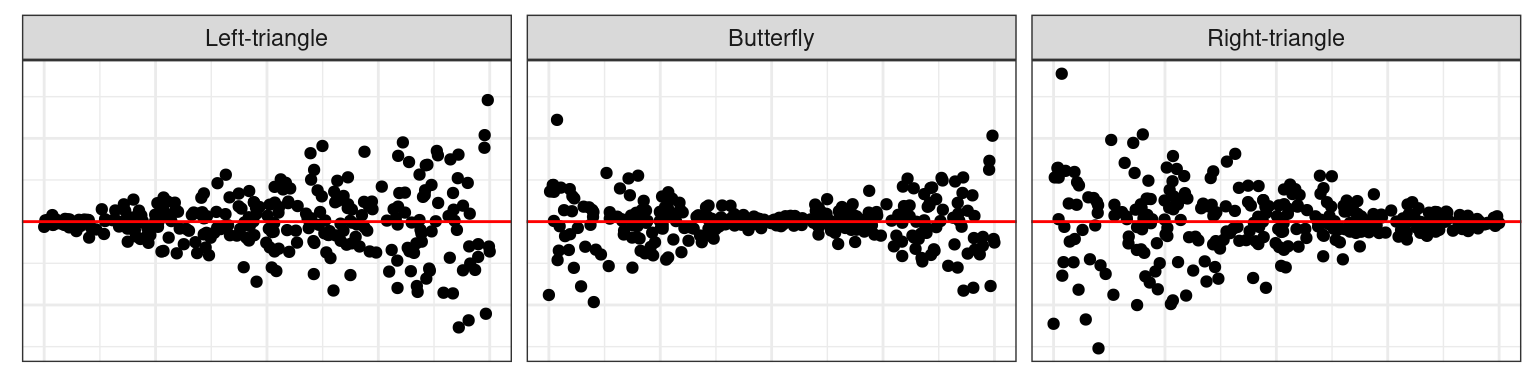
Heteroskedasticity
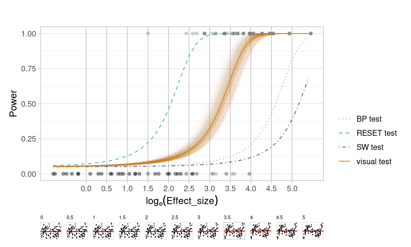
📏 Effect size: Non-linearity
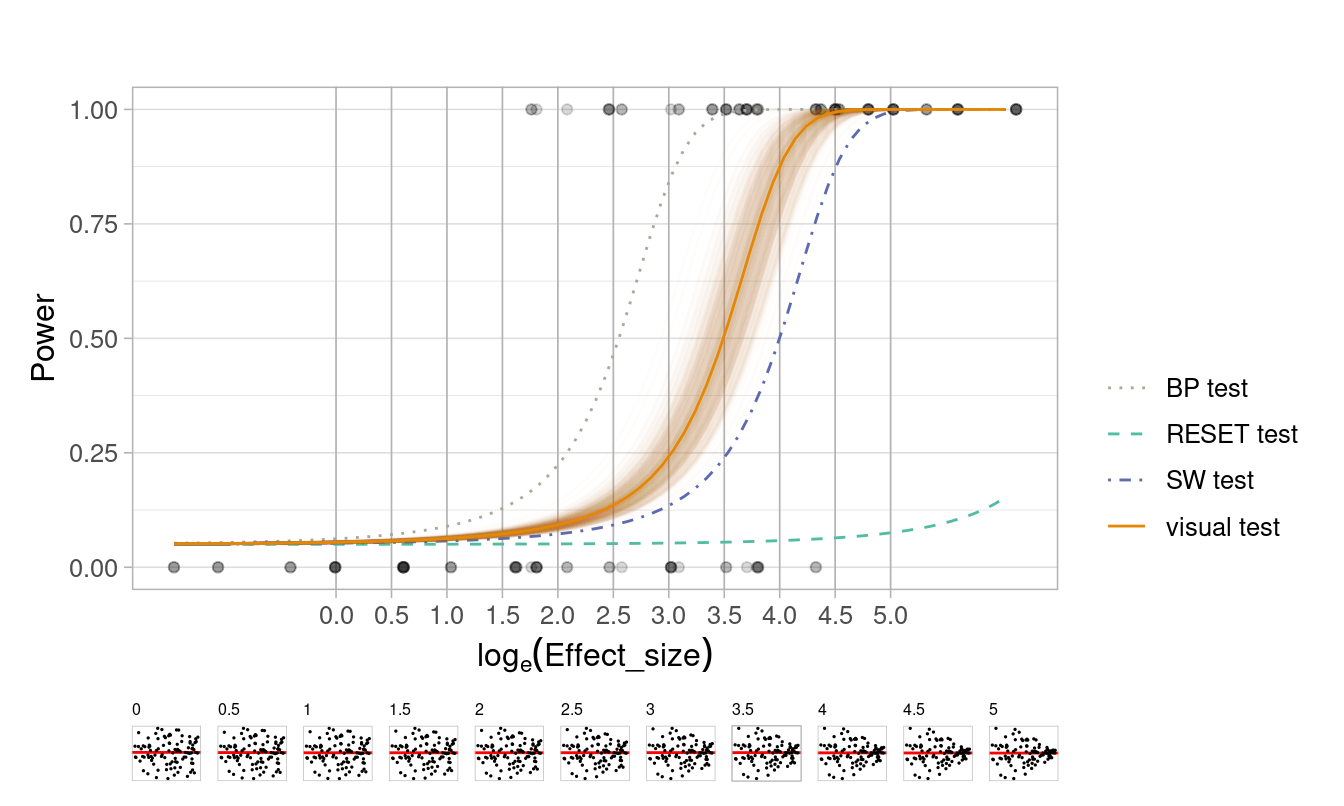
📏 Effect size: Heteroskedasticity
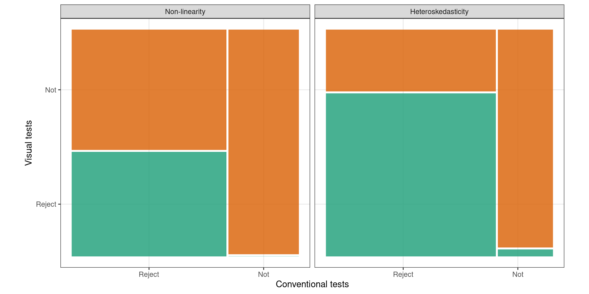
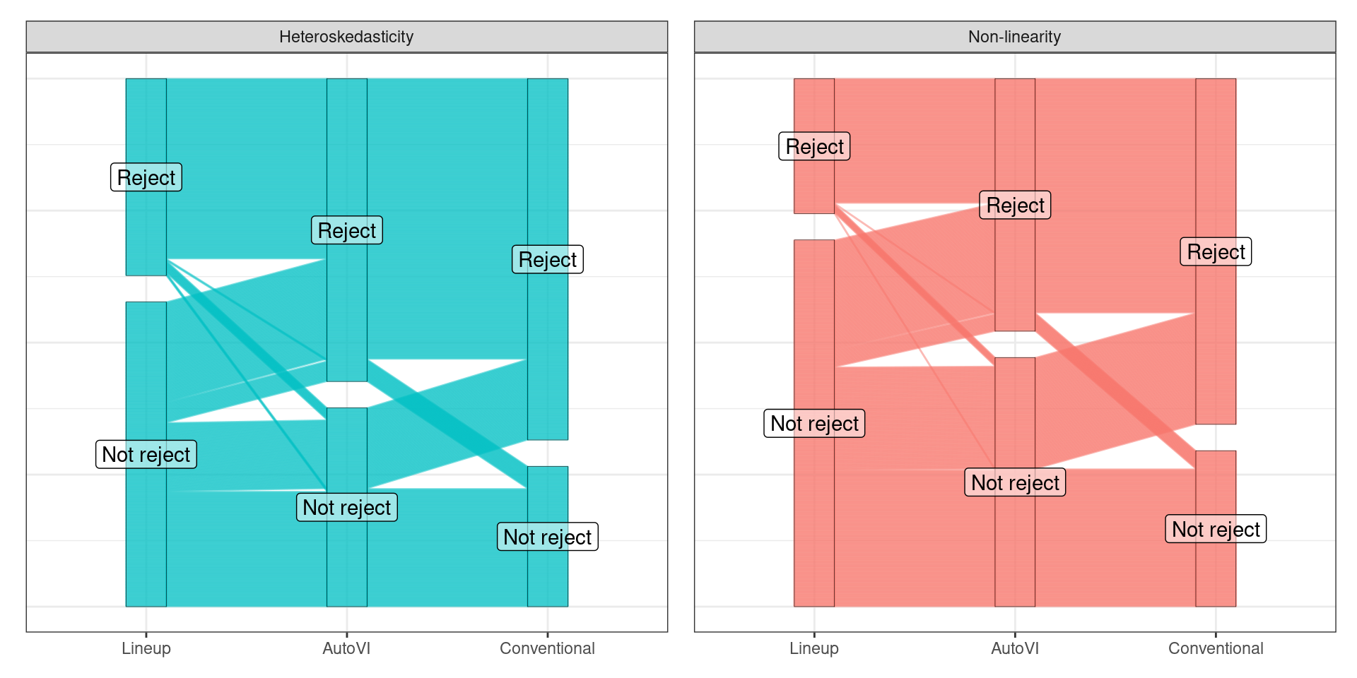
📊 Test Outcomes
🪩 The Oddball Dataset
⚠️ Limitations of Lineup Protocol
- Humans cannot (easily) evaluate
- lineups w/ many plots

- a large number of lineups
💡Training: Model Violations
Non-linearity + Heteroskedasticity
Non-normality + Heteroskedasticity
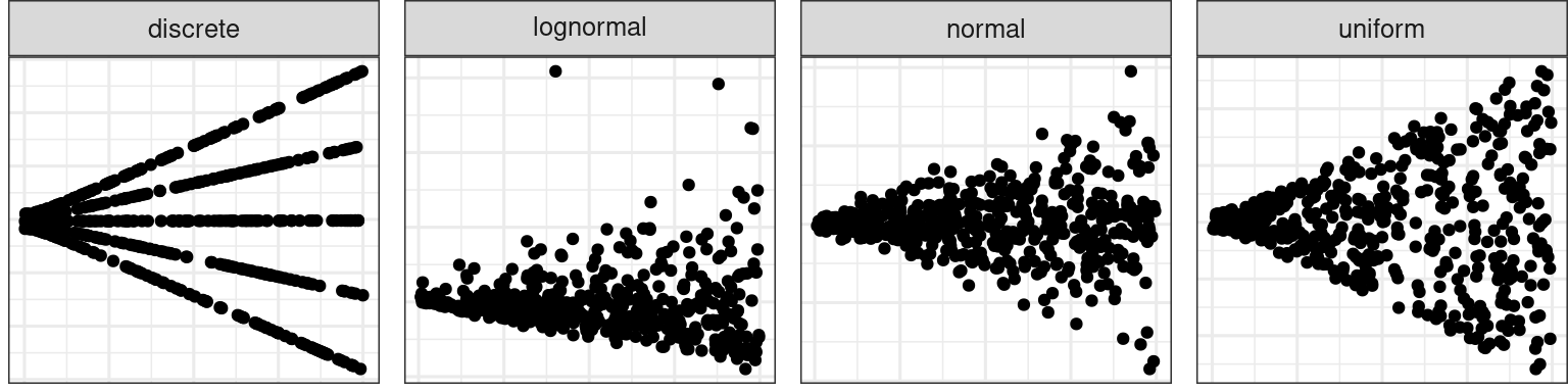
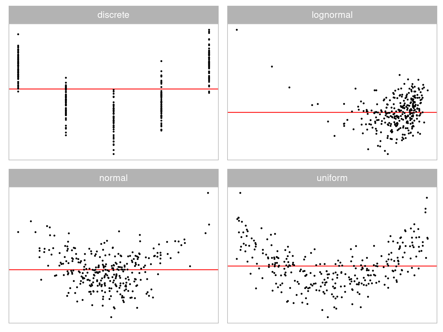
💡Training: Predictor Distribution
Distribution of predictor
Comparison to Visual Inference
💡Example: Boston Housing
autovi💡Example: Boston Housing
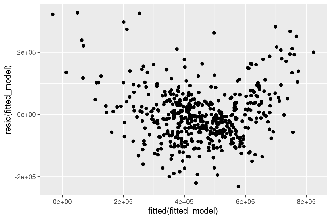
Null residuals are simulated from the fitted model assuming it is correctly specified.
checker <- auto_vi(fitted_model = fitted_model,
                   keras_model = get_keras_model("vss_phn_32"))
checker$rotate_resid()
# A tibble: 489 × 2
.fitted .resid
<dbl> <dbl>
1 632372. 24372.
2 525177. 13236.
3 646753. 54824.
4 624848. -98465.
5 611817. 188264.
6 551051. -67975.
7 504757. 142250.
8 445700. -175323.
9 281912. -101298.
10 453398. -121730.
# ℹ 479 more rows
:::
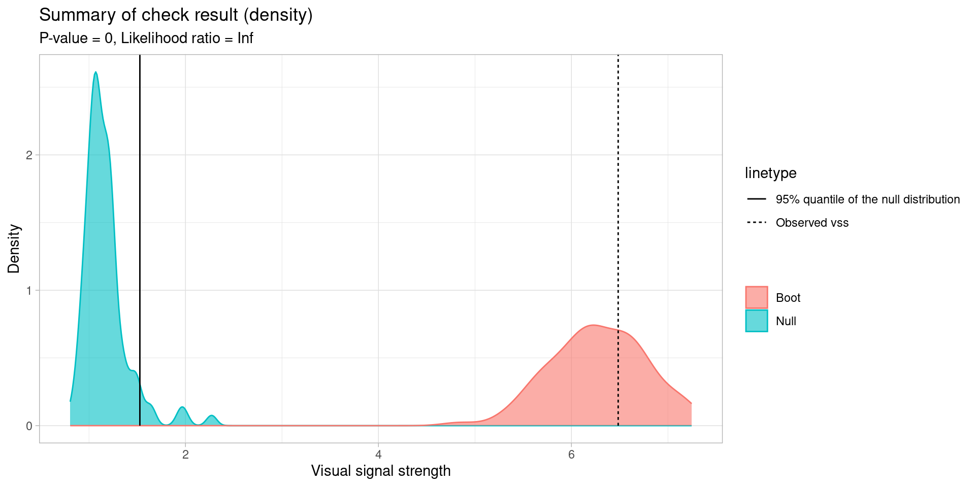
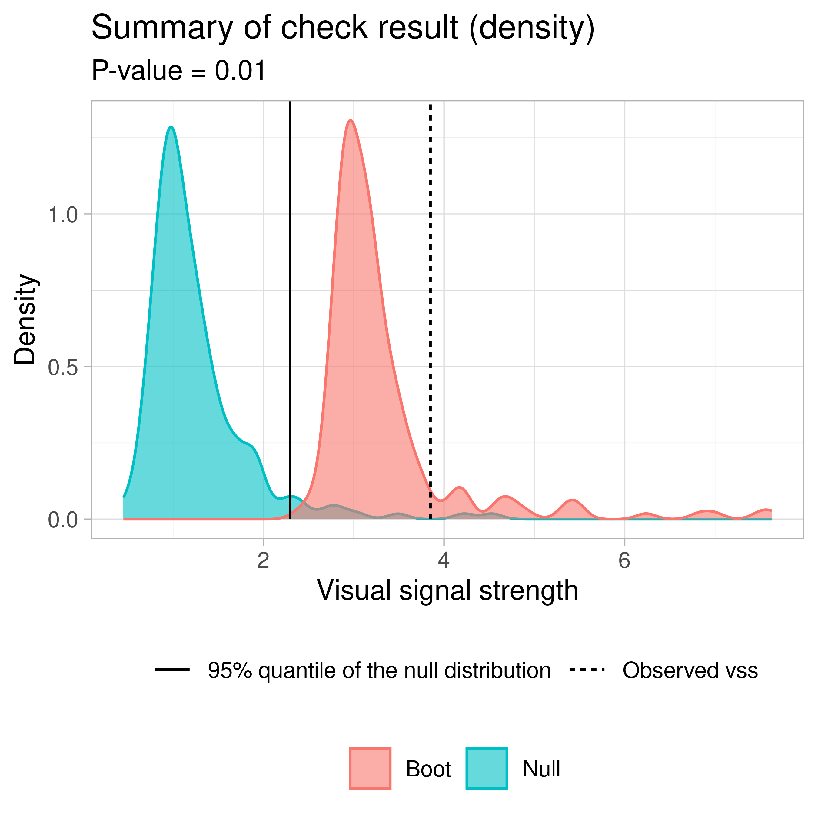
vss()
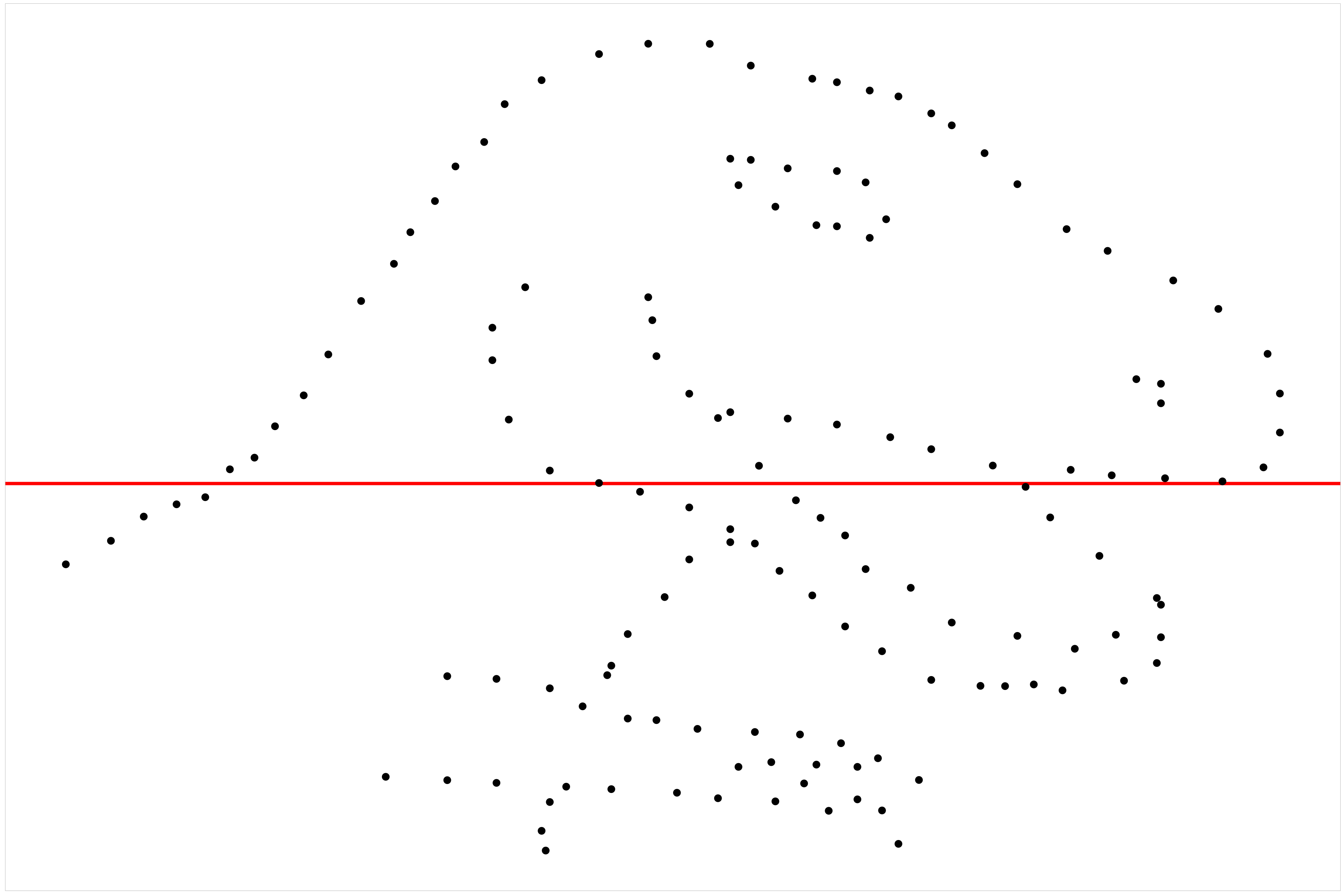
💡Example: Dinosaur
RESET \(p\)-value = 0.742
B-P \(p\)-value = 0.36
S-W \(p\)-value = 9.21e-05
:::
Thanks! Any questions?

Advisors


References

Belsley, David A., Edwin Kuh, and Roy E. Welsch. 1980. Regression Diagnostics: Identifying Influential Data and Sources of Collinearity. 14. [pr.]. Wiley Series in Probability and Mathematical Statistics. New York: Wiley.
Buja, Andreas, Dianne Cook, Heike Hofmann, Michael Lawrence, Eun-Kyung Lee, Deborah F Swayne, and Hadley Wickham. 2009. “Statistical Inference for Exploratory Data Analysis and Model Diagnostics.” Philosophical Transactions of the Royal Society of London A: Mathematical, Physical and Engineering Sciences 367 (1906): 4361–83. https://doi.org/10.1098/rsta.2009.0120.
Cook, R. Dennis, and Sanford Weisberg. 1982. “Criticism and Influence Analysis in Regression.” Sociological Methodology 13: 313–61. https://doi.org/10.2307/270724.
Draper, N. R., and H. Smith. 1998. Applied Regression Analysis. 1st ed. Wiley Series in Probability and Statistics. Hoboken, NJ: Wiley. https://books.google.com/books?id=d6NsDwAAQBAJ.
Mason, Harriet, Stuart Lee, Ursula Laa, and Dianne Cook. 2024. “Numbats/Cassowaryr.” NUMBATS: Non-Uniform Monash Business Analytics Team repo for joint projects. https://github.com/numbats/cassowaryr.
Montgomery, Douglas C., and Elizabeth A. Peck. 1982. Introduction to Linear Regression Analysis. Hoboken, NJ: John Wiley & Sons.
VanderPlas, Susan, Christian Röttger, Dianne Cook, and Heike Hofmann. 2021. “Statistical Significance Calculations for Scenarios in Visual Inference.” Stat 10 (1). https://doi.org/10.1002/sta4.337.