Animint:

Grammar of Graphics

Grammar of Graphics

        ggplot(data=profile, aes(x=height, fill=gender)) +
          geom_bar(aes(y=..count..), position="stack", stat="bin")

Animint

extends ggplot2 with interactive aesthetics

• clickSelects is an aesthetic which indicates which variable to use as a key when a plot object is clicked.
• showSelected is an aesthetic which indicates the variable to show in response to selection of a plot object.
• The combination of these two aesthetics allows us to create linked, interactive plots.

Animint

extends ggplot2 with interactive aesthetics

• Statistically, this allows us to interactively show conditional distributions (when the conditioning variable is categorical or discretized)
• Animint also adds other aesthetics to this framework: hoverSelects , tooltip , and time (for automatic iteration between cases, that is, animation)

Building Plots with Animint
and ggplot2

Demo Dataset

• Weather records from stations in Texas, Jan - July 2015
  From the Global Historical Climatology Network
• Multiple stations within a small area have been combined and labeled as the most central station in the region.

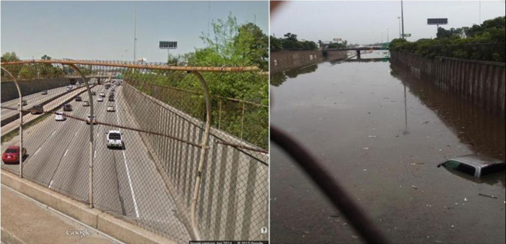
May 2015 flooding in Houston, TX

May 2015 flooding in Houston, TX

May 2015 flooding along the Blanco River (TX)

May 2015 flooding along the Blanco River (TX)

Building Plots with Animint and ggplot2

texasPrecipitation <- ggplot() +
  geom_tallrect(aes(xmin=min.day, xmax=max.day, clickSelects=week),
                data=statesummary, alpha=.1, fill="black", color="black") +
  geom_rect(aes(xmin=min.day, xmax=max.day, ymin=0, ymax=precip.median,
                clickSelects=week), data=statesummary) +
  geom_point(aes(x=day, y=precip.max), size=4, fill="transparent", color="black", data=statesummary) +
  geom_text(aes(x=ymd("2015-04-15"), y=16, label=label, showSelected=week), data=statesummary) +
  xlab("") + ylab("Weekly Precipitation (in)") +
  ggtitle("Precipitation across Texas, 2015") +
  theme_animint(width=350, height=540)

animint2dir(
  list(
  # list of all of the plots to 
  # render with animint
    precip = texasPrecipitation
  )
)

Building Plots with Animint and ggplot2

Interactivity within a single plot

Building Plots with Animint and ggplot2

Adding linked plots

texasOutline <- ggplot() +
  geom_path(data=rivers, aes(x=long, y=lat, group=group), color="grey", size=.5) +
  geom_polygon(data=lakes, aes(x=long, y=lat, group=group), fill="grey", size=.5) +
  geom_path(data=tx, aes(x=long, y=lat, group=group)) +
  theme(axis.line = element_blank(), axis.text = element_blank(),
        axis.ticks = element_blank(), axis.title = element_blank()) +
  theme_animint(width=600, height=540) # Size of the plot when rendered in HTML

Building Plots with Animint and ggplot2

Adding linked plots

weatherStations <- texasOutline + ggtitle("Weekly Precipitation") +
  geom_point(data=weathersummary,
             aes(x=longitude, y=latitude, # Standard aesthetics
                 showSelected=week, tooltip=station.name,# animint aes 
                 fill=precip.wk), color="black", size=4) +
             # animint specifies fill and color separately for points
  scale_fill_gradient2("Precip (in)", low="white", mid="steelblue1", midpoint=10, high="steelblue3")

Building Plots with Animint and ggplot2

Adding linked plots

Animint Internals

R to d3 compiler

(R code, runs once)

• Saves data file(s) for each plot layer
• Creates a JSON file which contains
  • Descriptions of each plot layer (aesthetic mappings, scales, ...)
  • Locations of data file(s) for each layer
  • A map of links between layers due to interactive aesthetics (clickSelects, hoverSelects, showSelected, tooltip, ...)
  • Theme information

Animint Renderer

(JavaScript code, runs in browser on page load)

• Downloads the JSON file using d3.json()
• Builds the plot, legend, and selectors
• Loads the data for each (currently selected/displayed) geom
• Draws selected geoms
• Re-draws geoms based on selection events

Animint Bindings

• HTML: animint2dir() saves an index.html file, required javascript files, the JSON plot description, and data to a local directory
• Gist: animint2gist() posts a gist to your github account (which can be viewed using http://bl.ocks.org/)
• knitr bindings: structure(..., class="animint") will create an interactive applet when knitting output to HTML
• shiny bindings: renderAnimint() and animintOutput() create an animint applet within a shiny app

Other Features

• Multiple selection: selector.types = list(station = "multiple")
• Tooltips: aes(tooltip = label)
• CSS ID variables: aes(id = idvar) allows for customization with CSS
• Links: aes(href = url) creates links that open in a new tab
• Transitions: aes(key = variable) creates smooth transitions
• Initial selector values: first = list(variable = value) will select "value" on initial load