| Factor | Df | Sum Sq | Mean Sq | F value | Pr(>F) |
|---|---|---|---|---|---|
| grade | 2 | 112 | 56.000000 | 26.25 | 1.26e-05 |
| Residuals | 15 | 32 | 2.133333 | ||
| Total | 17 | 144 |
A Short Overview of Statistics
What is Statistics?
The science of developing and studying methods for collecting, analyzing, interpreting, and presenting empirical data
- How should I conduct my experiment?
- What is the best way to test my hypothesis?
- What is the true value of ____
(and how precisely do I know that value)? - What does my experiment/sample tell me about my data?
- What is the future value of ____ given what I know now?

Statistical Tasks
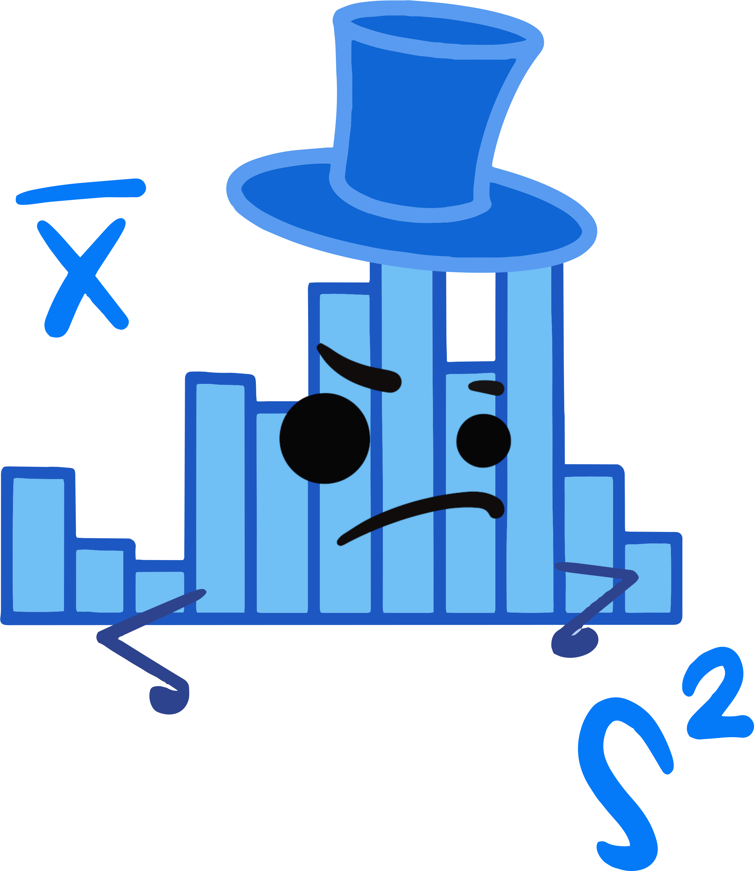
Description: What does the data say?
Statistical Tasks
Experimental Design: What’s the best way to collect data?

Statistical Tasks
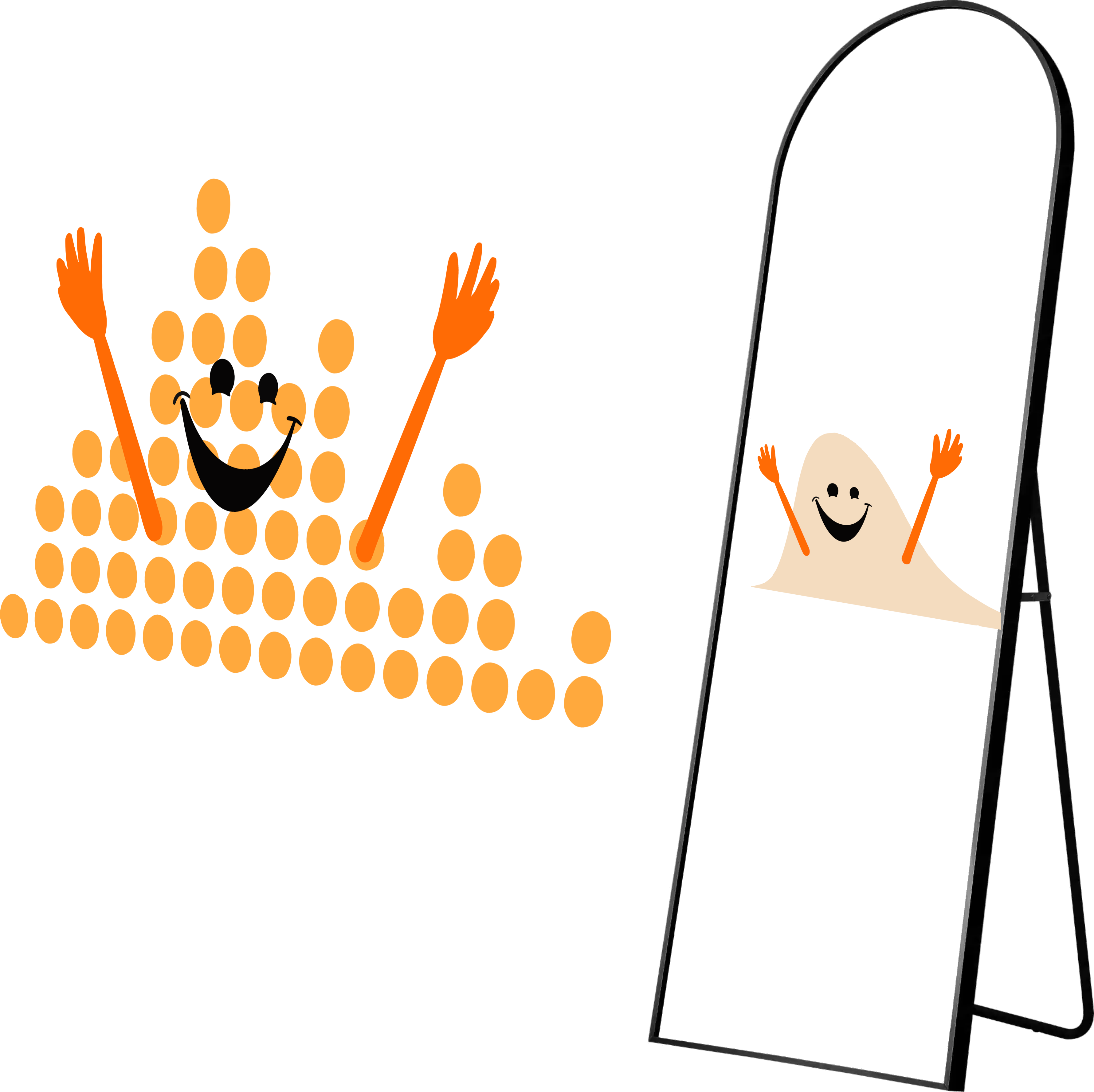
Inference: What does the data tell us (about the population)?
Statistical Tasks
Prediction: What will happen next?

An Historical Example
The Logic of Hypothesis Testing
Can someone tell whether tea or milk is added first to a cup?
4 cups of tea with milk first , 4 cups of tea with tea first
Randomize the order
Test the cups and make predictions for all 8 cups
What is the probability that someone gets all 8 correct?
A Lady Tasting Tea
If the 4 milk-first cups are correctly identified, so are the 4 tea-first cups
If we assume the taster is just guessing, we could just as easily flip 4 coins

A Lady Tasting Tea
Statistical evaluation
Null hypothesis: Taster is guessing
If our experimental results are likely to occur by random chance, we can’t really say whether the taster is guessing or not
We fail to reject the null hypothesisIf our experimental results are not likely to occur by random chance, we may decide it’s more likely that there is another explanation… the taster knows their stuff!
Try it out!
Go to https://shiny.srvanderplas.com/APL and start with the Tea Tasting tab.
What effect does the # simulations have on the results?
What effect does the # test cups have on the results?
- Assuming the number of observed cups is the same as the number of test cups
- Assuming the number of observed cups is less than the number of test cups
Hypothesis Testing Logic
Run an experiment and generate an observed value
Simulate a large number of experiments under random chance (the null hypothesis)
Compare the observed value to the results of the simulated experiments
Decide whether the observed value is plausible under random chance, or it is more likely that the results would happen if the null hypothesis is wrong
Theory-based Statistics
Run an experiment and generate a test statistic (t, z, F, \(\chi^2\))
Compare the observed value to the theoretical distribution
Decide whether the observed value is plausible under random chance, or it is more likely that the results would happen if the null hypothesis is wrong
Try it out
Go to https://shiny.srvanderplas.com/APL and start with the Distributions tab.
What changes when you change distribution?
How many samples do you need for the simulation histogram to look similar to the theoretical distribution?
What effect does setting your observed value to be larger have on the p-value?
Note: At this point, we are doing tests examining values greater than the observed value. This will obviously not always hold true.How different is the simulation p-value from the theoretical p-value? Does this change when you increase the number of samples?
Statistical Test Logic
Goal: Are the experiment results are compatible with the null hypothesis?
if the region that is “more extreme” than the observed value is very small, then the experimental results are surprising
- This suggests the null hypothesis might not be reliable
- Reject \(H_0\) in favor of the alternative
Statistical Test Logic

Statistical Test Logic
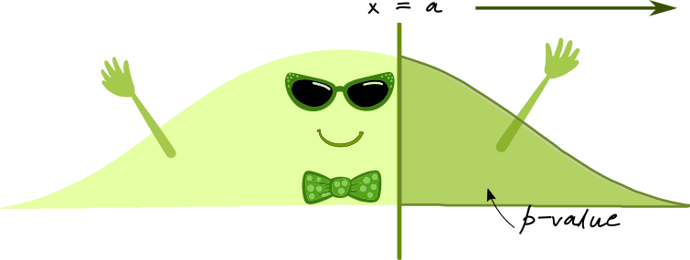
the region that is “more extreme” than the observed value is summarized as the p-value – the area of that region.
- p-values lower than \(\alpha = 0.05\), a pre-specified cutoff are considered “statistically significant”
that is, they should lead to a rejection of the null hypothesis
- p-values lower than \(\alpha = 0.05\), a pre-specified cutoff are considered “statistically significant”
Two Sided Tests
- If we don’t know/care whether \(x < a\) or \(x > a\), we use a two-sided test
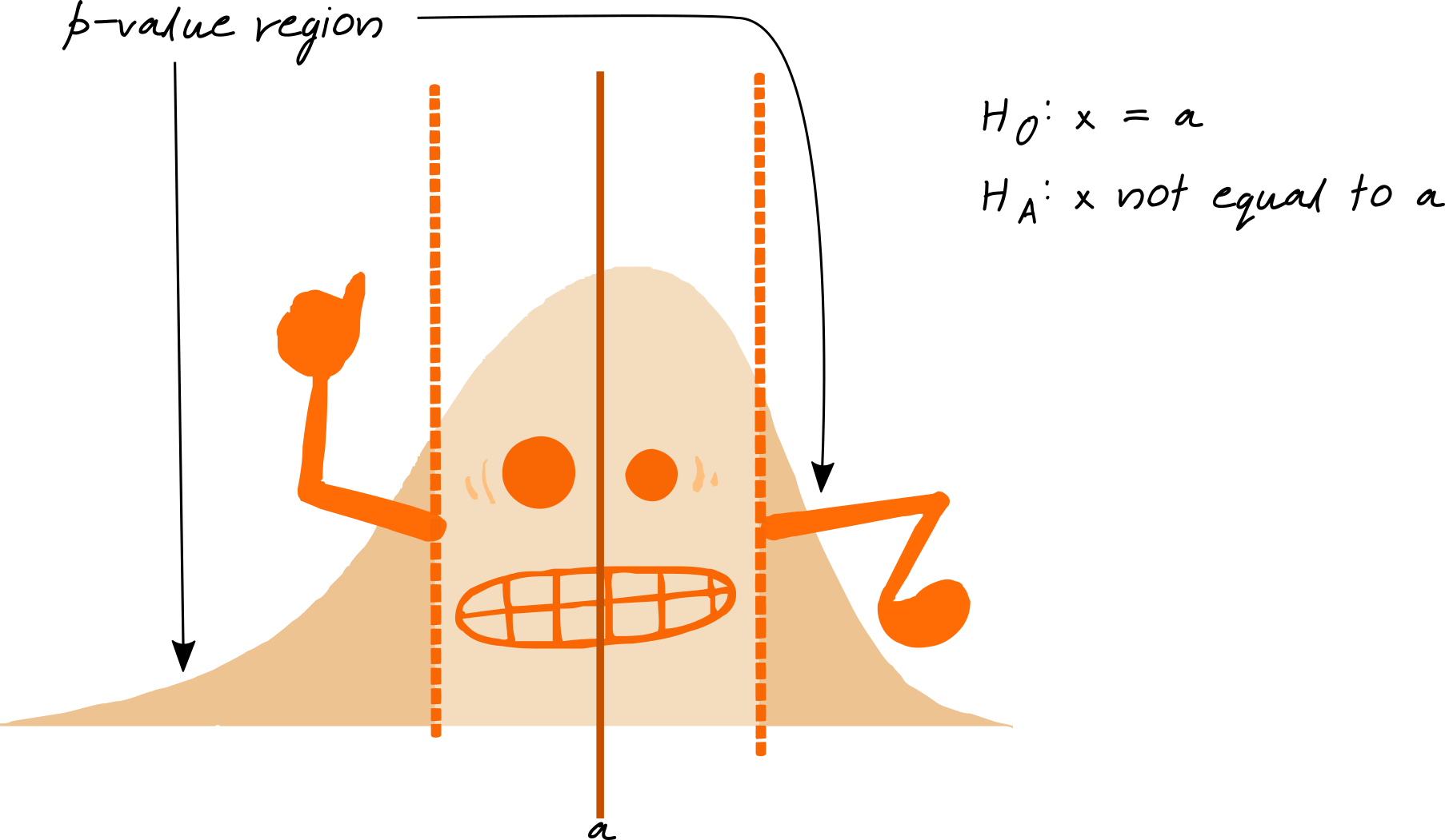
You can experiment with two-sided tests here:
https://shiny.srvanderplas.com/APL/ and click on “One Continuous Variable”
Confidence Intervals
Another way to use statistics is to get a range of “plausible” values based on the estimate + variability
This is called a confidence interval

Confidence Intervals
Every confidence interval has a “level” of \(1-\alpha\), just like every hypothesis test has a significance level \(\alpha\)
Confidence intervals with higher levels (e.g. .99 instead of .95) are wider
Interval width depends on
- sample size
- variability
- confidence level
A CI of (A, B) is read as “We are 95% confident that the true value of _________ lies between A and B”
Experimental Design
One Categorical Variable
Statistic: # Successes (out of # Trials)
Simulation method: Flip coins \((p = 0.5)\), weighted spinners \((p\neq 0.5)\)
Theoretical distribution: Binomial
https://shiny.srvanderplas.com/APL/ and click on “One Categorical Variable”
One Continuous Variable
- Statistic: \(\displaystyle t = \frac{\overline x - \mu}{s/\sqrt{n}}\) where
- \(\overline x\) is the sample mean,
- \(s\) is the sample standard deviation,
- \(\mu\) is the hypothesized mean, and
- \(n\) is the sample size
- Simulation method: none
- Theoretical distribution: \(t\) with \(n-1\) degrees of freedom
https://shiny.srvanderplas.com/APL/ and click on “One Continuous Variable”
Two-group Tests
Categorical variable: Group 1 or Group 2?
Continuous variable: Some measurement
Statistic: \(\overline x_1 - \overline x_2\)
Simulation method: shuffle group labels
Theoretical distribution: \(t\)
(degrees of freedom are a bit complicated)
https://shiny.srvanderplas.com/APL/ and click on “Categorical + Continuous Variables”
Two-group Tests
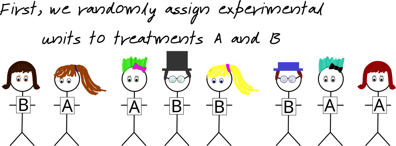
A two-sample experiment randomly divides up a sample of experimental units into two groups and calculates the sample mean for each group.
Two-group Tests
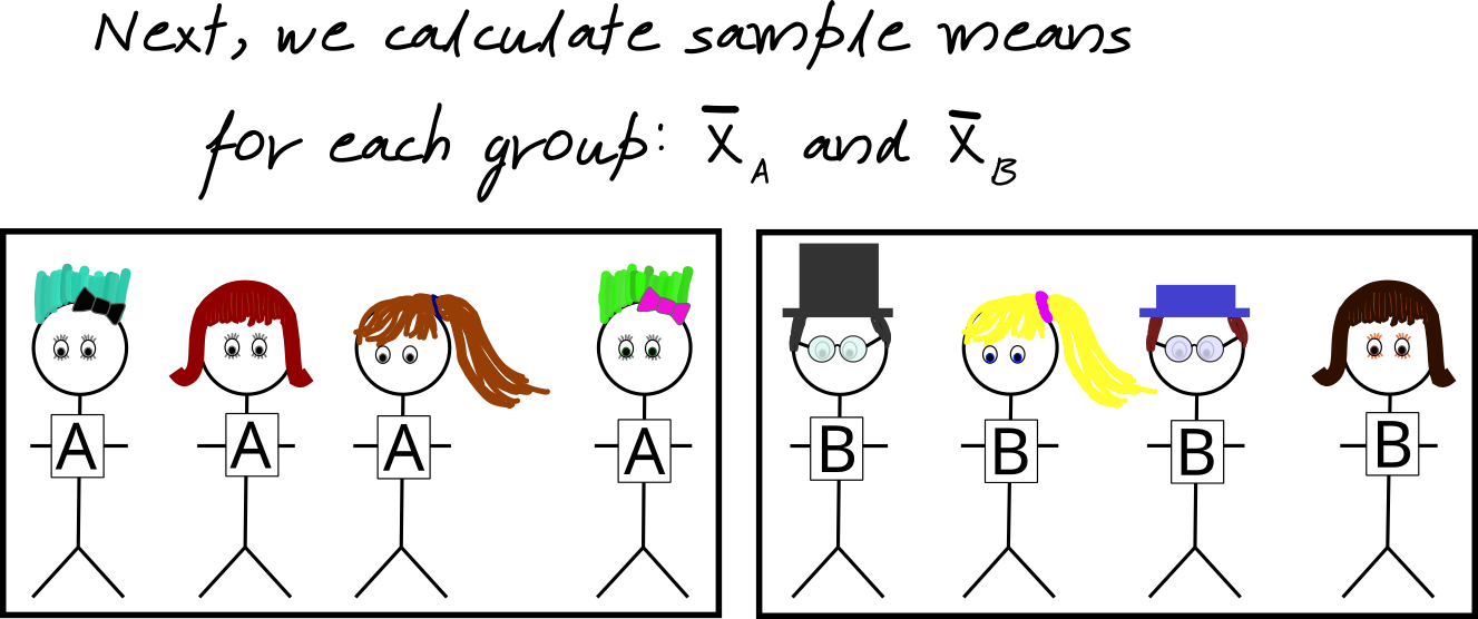
A two-sample experiment randomly divides up a sample of experimental units into two groups and calculates the sample mean for each group.
We compare \(\overline{X}_A\) and \(\overline {X}_B\): \(\overline{X}_A - \overline{X}_B\).
The standard deviation of \(\overline{X}_A - \overline{X}_B\) requires calculation: Use a two-sample test.
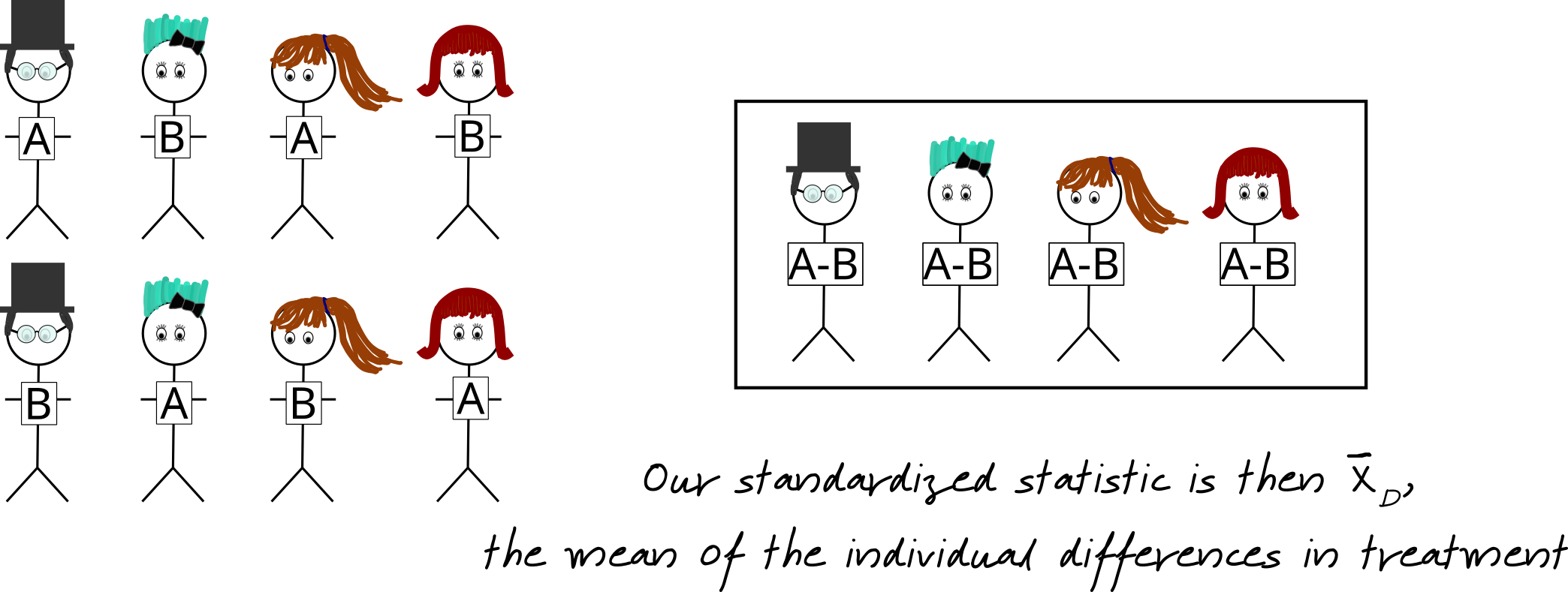
Repeated Measures
Repeated Measures
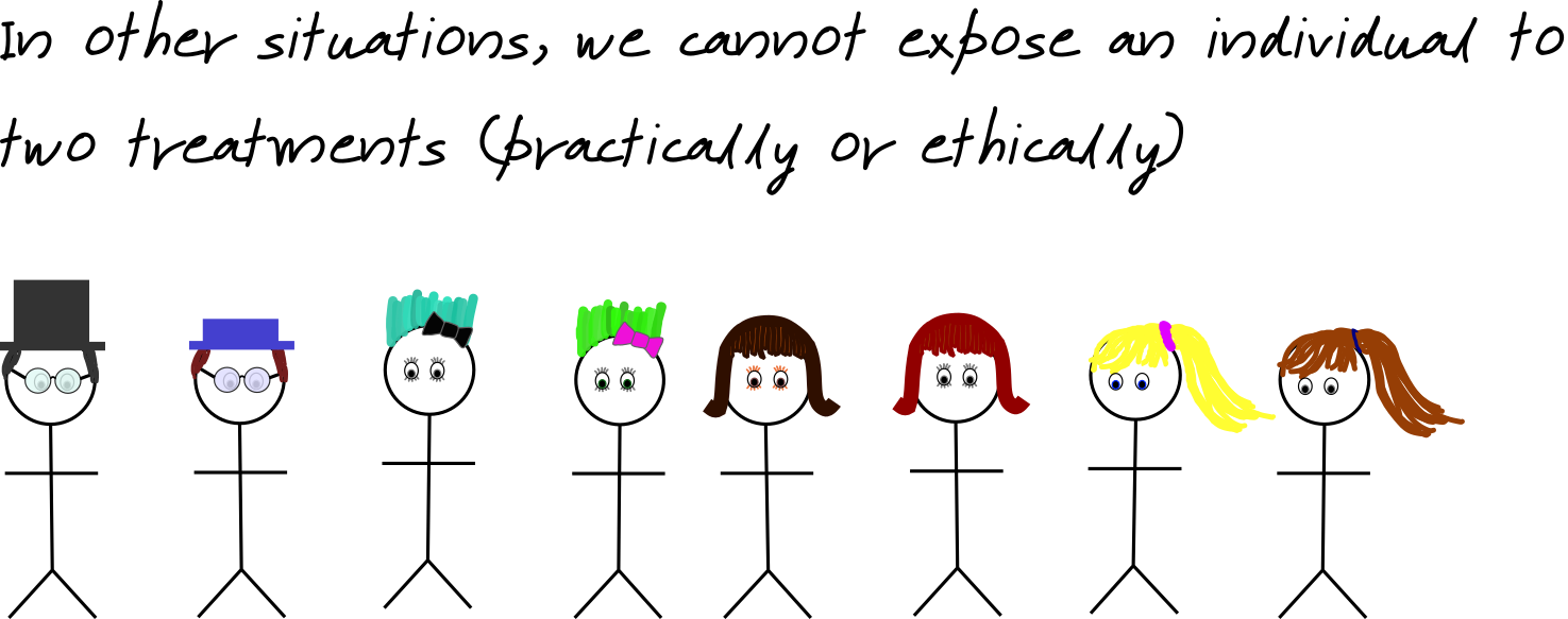
Matched Pairs
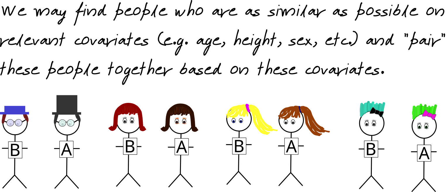
Matched Pairs
Matched Pairs
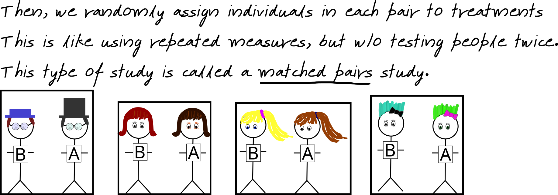
Matched Pairs

Analysis of Variance
Used for multiple groups
Suppose we have a group of schoolchildren separated by grade, and we want to examine the relationship between grade and height.

Analysis of Variance

If height is important, students in a single grade should be more similar than students across different grades.
Analysis of Variance
Goal: determine similarity within groups
within-groups sum-of-squares
Square the deviations from the group mean and add them upbetween-groups sum-of-squares
Sum of squared differences of the class average and the overall average for each student

Analysis of Variance
Results from ANOVA are shown in tables like this:
The F-value is the statistic, and is compared to an F(df1, df2) distribution - in this case, F(2, 15) to get a p-value.
Two Continuous Variables

We want to know if there is a linear association between x and y
Two Continuous Variables

If the slope of the line is nonzero, there is a linear association
Two Continuous Variables

We need to test whether that slope is significantly different from 0
Two Continuous Variables
Continuous variables: \(x\) and \(y\)
Statistic: \(a\), the sample slope
Simulation method: shuffle values of \(y\) relative to \(x\)
Theoretical distribution: \(t_{n-2}\), where \(n\) is the number of observations


