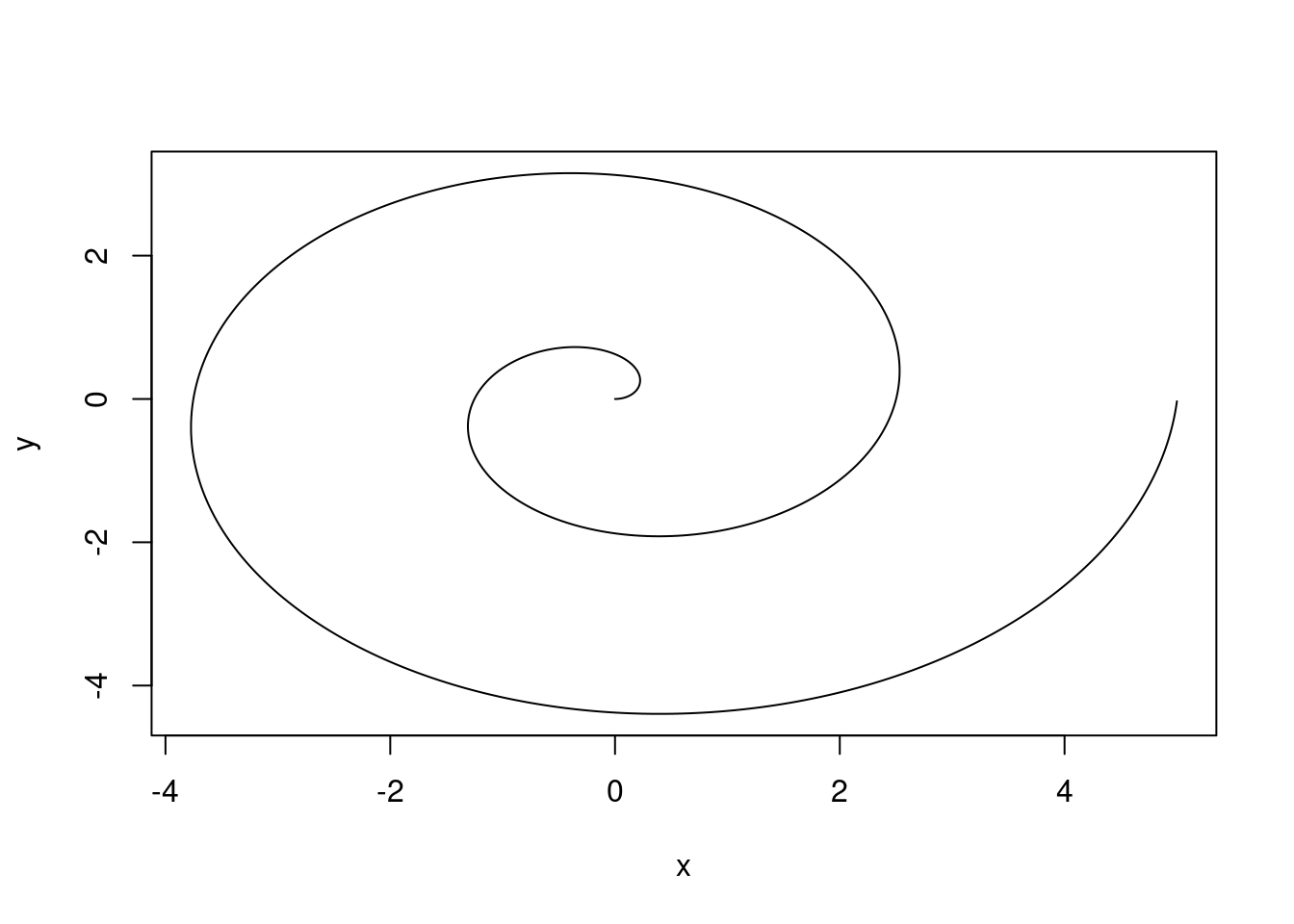
# Define the angle of the spiral (polar coords)
# go around two full times (2*pi = one revolution)
<- seq(0, 4*pi, .01)
theta # Define the distance from the origin of the spiral
# Needs to have the same length as theta
<- seq(0, 5, length.out = length(theta))
r
# Now define x and y in cartesian coordinates
<- r * cos(theta)
x <- r * sin(theta)
y
plot(x, y, type = "l")
2 Scripts and Notebooks
In this class, we’ll be using markdown notebooks to keep our code and notes in the same place. One of the advantages of both R and Python is that they are both scripting languages, but they can be used within notebooks as well. This means that you can have an R script file or a python script file, and you can run that file, but you can also create a document (like the one you’re reading now) that has code AND text together in one place. This is called literate programming and it is a very useful workflow both when you are learning programming and when you are working as an analyst and presenting results.
2.1 Scripts
Before I show you how to use literate programming, let’s look at what it replaces: scripts. Scripts are files of code that are meant to be run on their own. They may produce results, or format data and save it somewhere, or scrape data from the web – scripts can do just about anything.
Scripts can even have documentation within the file, using #
characters (at least, in R and python) at the beginning of a line. #
indicates a comment – that is, that the line does not contain code and should be ignored by the computer when the program is run. Comments are incredibly useful to help humans understand what the code does and why it does it.
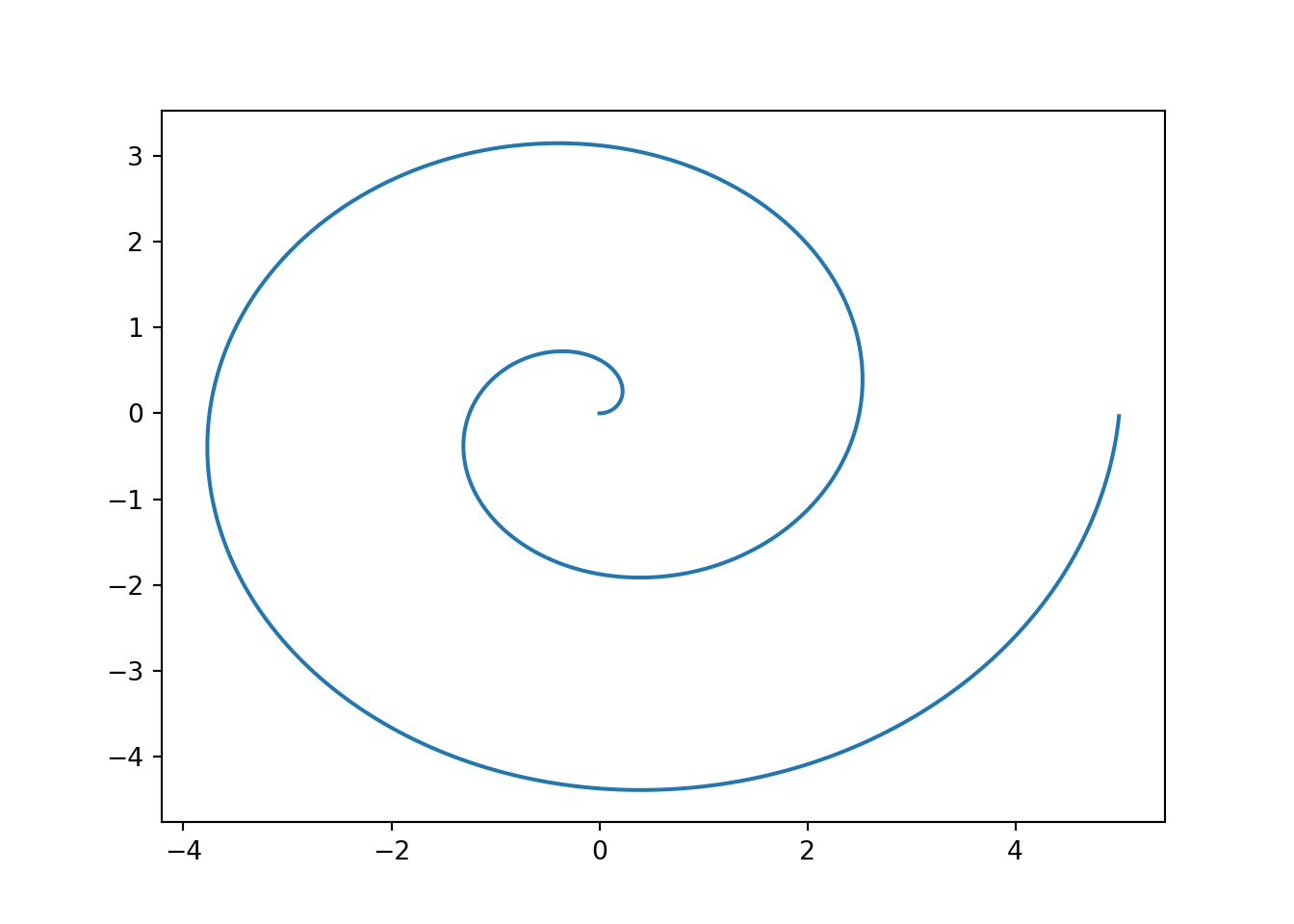
2.1.1 Plotting a logarithmic spiral
This code will use concepts we have not yet introduced - feel free to tinker with it if you want, but know that you’re not responsible for being able to write this code yet. You just need to read it and get a sense for what it does. I have heavily commented it to help with this process.
I have saved this script here. You can download it and open it up in RStudio (File -> Open -> Navigate to file location).
import numpy as np
import matplotlib.pyplot as plt
# Define the angle of the spiral (polar coords)
# go around two full times (2*pi = one revolution)
= np.arange(0, 4 * np.pi, 0.01)
theta # Define the distance from the origin of the spiral
# Needs to have the same length as theta
# (get length of theta with theta.size,
# and then divide 5 by that to get the increment)
= np.arange(0, 5, 5/theta.size)
r
# Now define x and y in cartesian coordinates
= r * np.cos(theta)
x = r * np.sin(theta)
y
# Define the axes
= plt.subplots()
fig, ax # Plot the line
ax.plot(x, y) plt.show()
I have saved this script here. You can download it and open it up in RStudio (File -> Open -> Navigate to file location).
Scripts can be run in Rstudio by clicking the Run button at the top of the editor window when the script is open.
2.1.2 Try it out!
Download the R and python scripts in the above example, open them in RStudio, and run each script using the Run button. What do you see?
(Advanced) Open a terminal in RStudio (Tools -> Terminal -> New Terminal) and see if you can run the R script from the terminal using
R CMD BATCH path/to/file/markdown-spiral-script.R
(You will have to modify this command to point to the file on your machine)
Notice that two new files appear in your working directory:Rplots.pdf
andmarkdown-spiral-script.Rout
(Advanced) Open a terminal in RStudio (Tools -> Terminal -> New Terminal) and see if you can run the R script from the terminal using
python3 path/to/file/markdown-spiral-script.py
(You will have to modify this command to point to the file on your machine)
This will require you to have python3 accessible to you on the command line, which may be a challenge if it is not set up in the way that I’m assuming it is. Feel free to make an appointment to see if we can figure it out, if this does not work the first time.
Most of the time, you will run scripts interactively - that is, you’ll be sitting there watching the script run and seeing what the results are as you are modifying the script. However, one advantage to scripts over notebooks is that it is easy to write a script and schedule it to run without supervision to complete tasks which may be repetitive. I have a script that runs daily at midnight, 6am, noon, and 6pm to pull information off of the internet for a dataset I’m maintaining. I’ve set it up so that this all happens automatically and I only have to check the results when I am interested in working with that data.
2.2 Notebooks
Notebooks are an implementation of literate programming. Both R and python have native notebooks that are cross-platform and allow you to code in R or python. This book is written using Quarto markdown, which is an extension of Rmarkdown, but it is also possible to use jupyter notebooks to write R code.
In this class, we’re going to use Quarto/R markdown, because it is a much better tool for creating polished reports than Jupyter (in my opinion). This matters because the goal is that you learn something useful for your own coding and then you can easily apply it when you go to work as an analyst somewhere to produce impressive documents. Jupyter notebooks are great for interactive coding, but aren’t so wonderful for producing polished results. They also don’t allow you to switch between languages mid-notebook, and since I’m trying to teach this class in both R and python, I want you to have both languages available.
There are some excellent opinions surrounding the use of notebooks in data analysis:
- Why I Don’t Like Notebooks” by Joel Grus at JupyterCon 2018
- The First Notebook War by Yihui Xie (response to Joel’s talk).
Yihui Xie is the person responsible forknitr
andRmarkdown
.
2.2.1 Try it out
Take a look at the R markdown sample file I’ve created to go with the R script above. You can see the HTML file it generates here.
Download the Rmd file and open it with RStudio.
Change the output to
output: word_document
and hit the Render button. Can you find the markdown-demo.docx file that was generated? What does it look like?
Change the output to
output: pdf_document
and hit the Render button. Can you find the markdown-demo.pdf file that was generated? What does it look like?
Rmarkdown tries very hard to preserve your formatted text appropriately regardless of the output document type. While things may not look exactly the same, the goal is to allow you to focus on the content and the formatting will “just work”.
Take a look at the jupyter notebook sample file I’ve created to go with the R script above. You can see the HTML file it generates here.
Download the ipynb file and open it with jupyter.
Export the notebook as a pdf file (File -> Save as -> PDF via HTML). Can you find the jupyter-demo.pdf file that was generated? What does it look like?
Export the notebook as an html file (File -> Save as -> HTML). Can you find the jupyter-demo.html file that was generated? What does it look like?
The nice thing about quarto is that it will work with python and R seamlessly, and you can compile the document using python or R. R markdown will also allow you to use python chunks, but you must compile the document in R.
Take a look at the Qmd notebook sample file I’ve created to go with the scripts above. You’ll notice that it is basically the script portion of this textbook – that’s because I’m writing the textbook in Quarto.
Download the qmd file and open it with RStudio
Try to compile the file by hitting the Render button
(Advanced) In the terminal, type in
quarto render path/to/file/quarto-demo.qmd
. Does that render the HTML file? One advantage of this is that using quarto to render the file doesn’t require R at the command line. As the document contains R chunks, R is still required to compile the document, but the biggest difference between qmd and rmd is that qmd files are workflow agnostic - you can generate them in e.g. MS Visual Studio Code, compile them in that workflow, and never have to use RStudio.