SURF-based Keypoint Alignment

Susan VanderPlas

2018-09-24

The R code underlying the functions in this vignette were borrowed with permission from Vinces Gaitan’s blog post: https://www.kaggle.com/vicensgaitan/image-registration-the-r-way/notebook

I have modified the code where necessary in order to make it more pipeline-friendly and function oriented.

imlinks <- system.file(package = "ShoeSampleData", "extdata/") %>%
  list.files(pattern = "036285L", full.names = T) %>%
  sort()

clean_shoe_img <- function(im) {
  suppressMessages({
    im_bbox <- im %>%
      imsplit(axis = "c") %>%
      (function(x) is.finite((x[[1]] + x[[2]]) / x[[3]])) %>%
      as.cimg() %>%
      (function(x) x == 1)

    crop.bbox(im, im_bbox) %>%
      grayscale() %>%
      map_halfimg(fun = autocrop) %>%
      crop.borders(nx = 5, ny = 5) %>%
      autocrop() %>%
      threshold() %>%
      shrink(3) %>%
      grow(3) %>%
      autocrop() %>%
      # img_rotate_refit() %>%
      # magrittr::extract2("img") %>%
      grayscale()
  })
}

img_a <- load.image(imlinks[1]) %>% clean_shoe_img()
img_b <- load.image(imlinks[2]) %>% clean_shoe_img()
plot(imlist(img_a, img_b))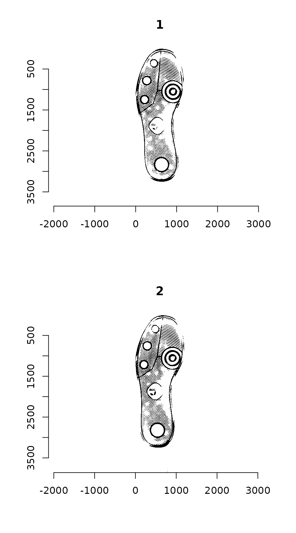

Image which will be used throughout this tutorial

We need to pad image a so that it is the same size as image b:

dim(img_a)
# [1] 1179 3847    1    1
dim(img_b)
# [1] 1196 3860    1    1
pad_size <- dim(img_b) - dim(img_a)
img_a <- pad(img_a, nPix = pad_size[1], axes = "x", pos = 1, val = max(img_a)) %>%
  pad(nPix = pad_size[2], axes = "y", pos = 1, val = max(img_a))

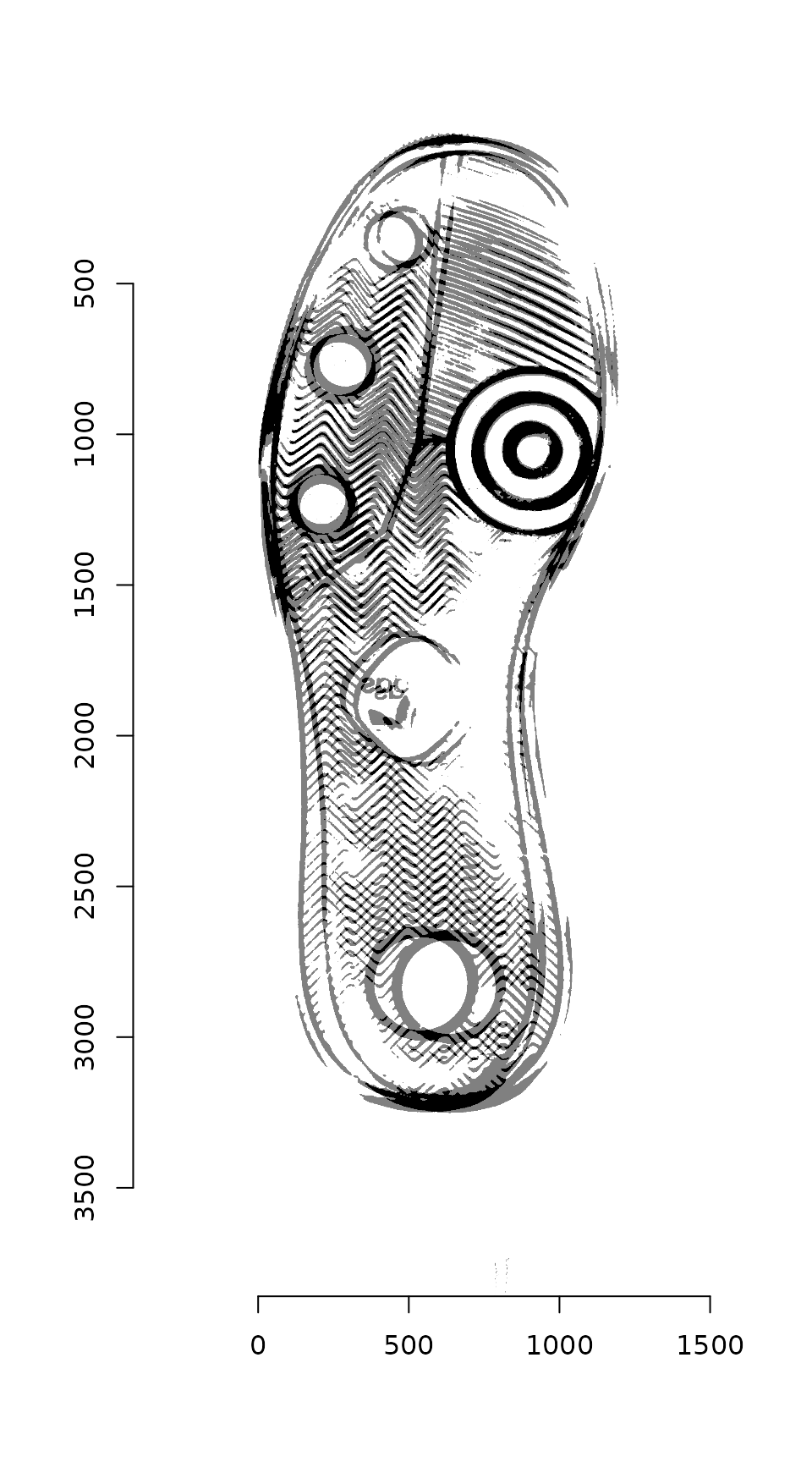
We can then overlay the two images to see how far apart they are:

plot(img_a + img_b)

Step 1: Keypoint Detection

Use the image_surf() function in the image.dlib package to identify keypoints for alignment

if (!"image.dlib" %in% installed.packages()) {
  devtools::install_github("bnosac/image/image.dlib")
}
library(image.dlib)
# image_surf requires a bmp file... 

get_surf <- function(im, n = 500) {
  tmpbmp <- tempfile(fileext = ".bmp")
  save.image(im, tmpbmp)
  image_surf(tmpbmp, max_points = 500)
}

sp_a <- get_surf(img_a)
sp_b <- get_surf(img_b)

centers_a <- data_frame(mx = sp_a$x, my = sp_a$y)
centers_b <- data_frame(mx = sp_b$x, my = sp_b$y)

kpf_a <- sp_a$surf
kpf_b <- sp_b$surf

With SURF, we can skip the image orientation and feature detection steps, as features are generated with an angle as part of the SURF algorithm.

Step 2: Match points

Match points are calculated using the K nearest neighbors algorithm, combined with some thresholding by distance.

match_points <- knn_points(kpf_a, kpf_b, centers_a, centers_b, show_plot = F)

Step 5: RANSAC

RANSAC is then used to find points that have similar homography.

ransac_points <- ransac(match_points$points_a, match_points$points_b)

par(mfrow = c(1, 2))

plot(img_a)
centers_a %$% points(mx, my, col = "orange")
points(match_points$points_a[ransac_points$inliers, ], col = "purple", pch = 16)
plot(img_b)
centers_b %$% points(mx, my, col = "orange")
points(match_points$points_b[ransac_points$inliers, ], col = "purple", pch = 16)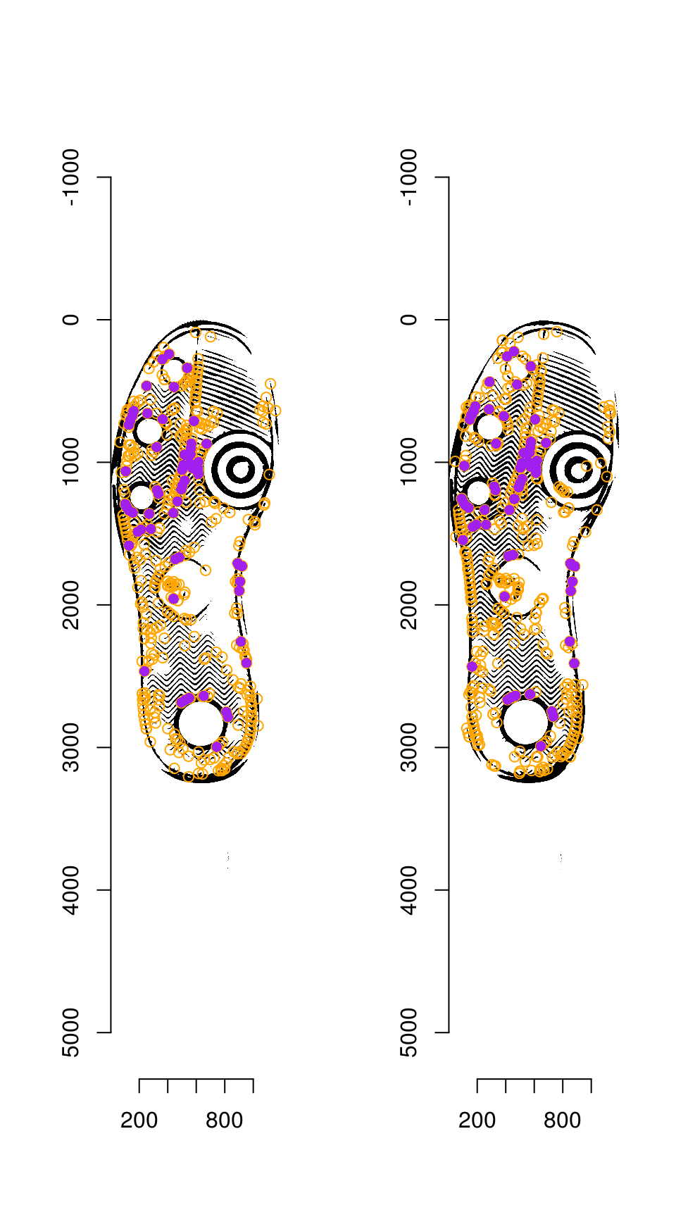

Step 6: Image Warping

The homography can be used to warp one image onto the other:

map_fcn <- map_affine_gen(ransac_points$homography)

img_a_warp <- imwarp(img_a, map_fcn, direction = "backward", boundary = "neumann")

plot(img_a_warp)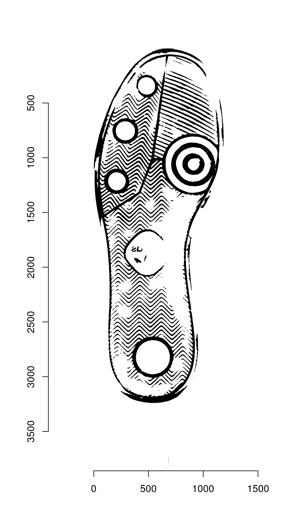

We can then overlay the two images:

blank_channel <- as.cimg(img_b > 0 & img_a_warp > 0)
overlaid_images <- imappend(imlist(img_a_warp, blank_channel, img_b), axis = "c")
plot(overlaid_images)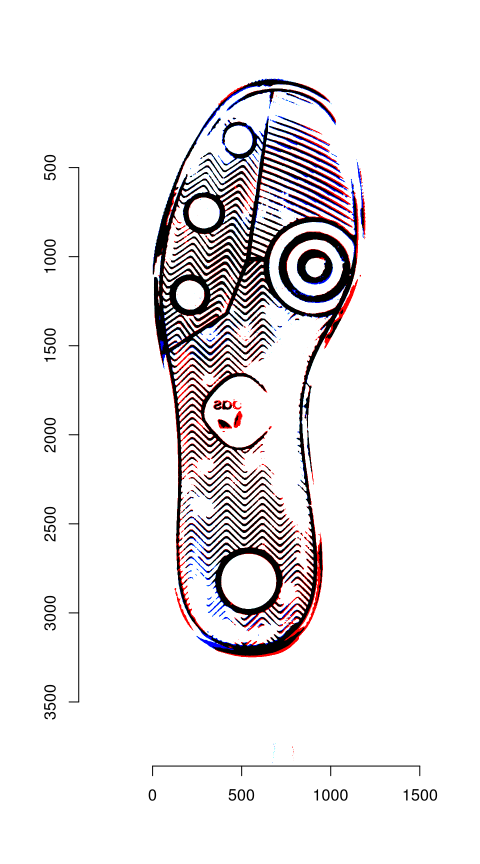

Areas that are in the first image only are shown in red; areas in the second image only are shown in blue. Areas in both images are shown in black.