library(dplyr)
data(starwars)
starwars
## # A tibble: 87 × 14
##    name     height  mass hair_color skin_color eye_color birth_year sex   gender
##    <chr>     <int> <dbl> <chr>      <chr>      <chr>          <dbl> <chr> <chr>
##  1 Luke Sk…    172    77 blond      fair       blue            19   male  mascu…
##  2 C-3PO       167    75 <NA>       gold       yellow         112   none  mascu…
##  3 R2-D2        96    32 <NA>       white, bl… red             33   none  mascu…
##  4 Darth V…    202   136 none       white      yellow          41.9 male  mascu…
##  5 Leia Or…    150    49 brown      light      brown           19   fema… femin…
##  6 Owen La…    178   120 brown, gr… light      blue            52   male  mascu…
##  7 Beru Wh…    165    75 brown      light      blue            47   fema… femin…
##  8 R5-D4        97    32 <NA>       white, red red             NA   none  mascu…
##  9 Biggs D…    183    84 black      light      brown           24   male  mascu…
## 10 Obi-Wan…    182    77 auburn, w… fair       blue-gray       57   male  mascu…
## # ℹ 77 more rows
## # ℹ 5 more variables: homeworld <chr>, species <chr>, films <list>,
## # vehicles <list>, starships <list>22 Data Cleaning
Objectives
- Identify required sequence of steps for data cleaning
- Describe step-by-step data cleaning process in lay terms appropriately
- Apply data manipulation verbs to prepare data for analysis
- Understand the consequences of data cleaning steps for statistical analysis
- Create summaries of data appropriate for analysis or display using data manipulation techniques
22.1 Introduction
In this section, we’re going start learning how to work with data. Generally speaking, data doesn’t come in a form suitable for analysis1 - you have to clean it up, create the variables you care about, get rid of those you don’t care about, and so on.

Some people call the process of cleaning and organizing your data “data wrangling”, which is a fantastic way to think about chasing down all of the issues in the data.
In R, we’ll be using the tidyverse for this. It’s a meta-package (a package that just loads other packages) that collects packages designed with the same philosophy2 and interface (basically, the commands will use predictable argument names and structure). You’ve already been introduced to parts of the tidyverse - specifically, readr and ggplot2.
dplyr (one of the packages in the tidyverse) creates a “grammar of data manipulation” to make it easier to describe different operations. I find the dplyr grammar to be extremely useful when talking about data operations, so I’m going to attempt to show you how to do the same operations in R with dplyr, and in Python (without the underlying framework).
Each dplyr verb describes a common task when doing both exploratory data analysis and more formal statistical modeling. In all tidyverse functions, data comes first – literally, as it’s the first argument to any function. In addition, you don’t use df$variable to access a variable - you refer to the variable by its name alone (“bare” names). This makes the syntax much cleaner and easier to read, which is another principle of the tidy philosophy.
In Python, most data manipulation tasks are handled using pandas[1]. In the interests of using a single consistent “language” for describing data manipulation tasks, I’ll use the tidyverse “verbs” to describe operations in both languages. The goal of this is to help focus your attention on the essentials of the operations, instead of the specific syntax.
There is also the datar python package[2], which attempts to port the dplyr grammar of data wrangling into python. While pandas tends to be fairly similar to base R in basic operation, datar may be more useful if you prefer the dplyr way of handling things using a data-first API.
I haven’t had the chance to add the datar package to this book, but it looks promising and may be worth your time to figure out. It’s a bit too new for me to teach right now - I want packages that will be maintained long-term if I’m going to teach them to others.
Note
There is an excellent dplyr cheatsheet available from RStudio. You may want to print it out to have a copy to reference as you work through this chapter.
Here is a data wrangling with pandas cheatsheet that is formatted similarly to the dplyr cheat sheet.
22.2 Tidy Data
There are infinitely many ways to configure “messy” data, but data that is “tidy” has 3 attributes:
- Each variable has its own column
- Each observation has its own row
- Each value has its own cell
These attributes aren’t sufficient to define “clean” data, but they work to define “tidy” data (in the same way that you can have a “tidy” room because all of your clothes are folded, but they aren’t clean just because they’re folded; you could have folded a pile of dirty clothes).
We’ll get more into how to work with different “messy” data configurations in Chapter 24 and Chapter 26, but it’s worth keeping rules 1 and 3 in mind while working through this module.
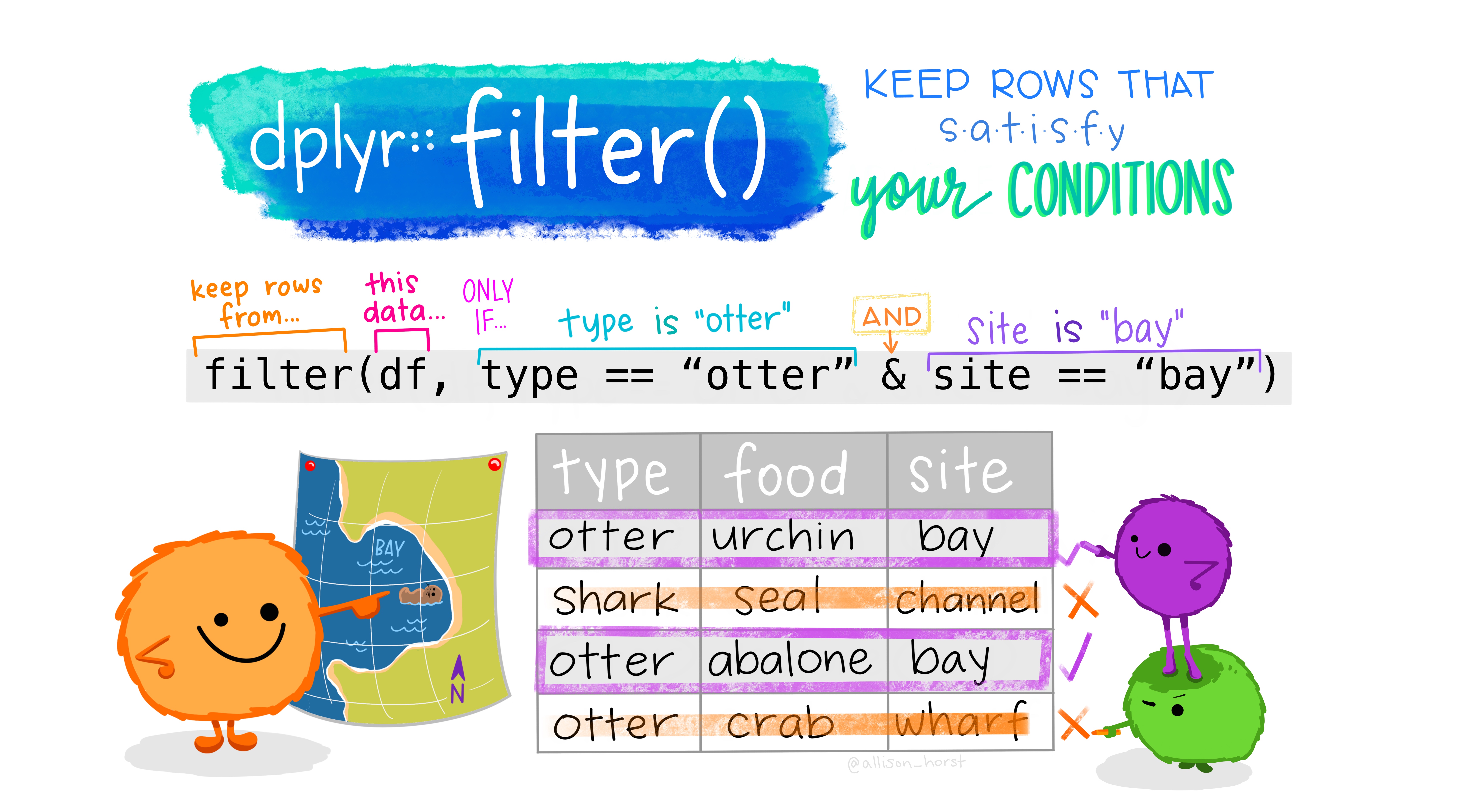
22.3 Filter: Subset rows
Filter allows us to work with a subset of a larger data frame, keeping only the rows we’re interested in. We provide one or more logical conditions, and only those rows which meet the logical conditions are returned from filter(). Note that unless we store the result from filter() in the original object, we don’t change the original.
Example: starwars
Let’s explore how it works, using the starwars dataset, which contains a comprehensive list of the characters in the Star Wars movies.
In the interests of demonstrating the process on the same data, I’ve exported the starwars data to a CSV file using the readr package. I had to remove the list-columns (films, vehicles, starships) because that format isn’t supported by CSV files. You can access the csv data here.
This data set is included in the dplyr package, so we load that package and then use the data() function to load dataset into memory. The loading isn’t complete until we actually use the dataset though… so let’s print the first few rows.
We have to use the exported CSV data in python.
import pandas as pd
starwars = pd.read_csv("https://github.com/srvanderplas/datasets/raw/main/clean/starwars.csv")
starwars
##               name  height   mass  ...     gender homeworld species
## 0   Luke Skywalker   172.0   77.0  ...  masculine  Tatooine   Human
## 1            C-3PO   167.0   75.0  ...  masculine  Tatooine   Droid
## 2            R2-D2    96.0   32.0  ...  masculine     Naboo   Droid
## 3      Darth Vader   202.0  136.0  ...  masculine  Tatooine   Human
## 4      Leia Organa   150.0   49.0  ...   feminine  Alderaan   Human
## ..             ...     ...    ...  ...        ...       ...     ...
## 82             Rey     NaN    NaN  ...   feminine       NaN   Human
## 83     Poe Dameron     NaN    NaN  ...  masculine       NaN   Human
## 84             BB8     NaN    NaN  ...  masculine       NaN   Droid
## 85  Captain Phasma     NaN    NaN  ...        NaN       NaN     NaN
## 86   Padmé Amidala   165.0   45.0  ...   feminine     Naboo   Human
##
## [87 rows x 11 columns]

from skimpy import skim
skim(starwars)
## ╭─────────────────────────────── skimpy summary ───────────────────────────────╮
## │          Data Summary                Data Types                              │
## │ ┏━━━━━━━━━━━━━━━━━━━┳━━━━━━━━┓ ┏━━━━━━━━━━━━━┳━━━━━━━┓                       │
## │ ┃ Dataframe         ┃ Values ┃ ┃ Column Type ┃ Count ┃                       │
## │ ┡━━━━━━━━━━━━━━━━━━━╇━━━━━━━━┩ ┡━━━━━━━━━━━━━╇━━━━━━━┩                       │
## │ │ Number of rows    │ 87     │ │ string      │ 8     │                       │
## │ │ Number of columns │ 11     │ │ float64     │ 3     │                       │
## │ └───────────────────┴────────┘ └─────────────┴───────┘                       │
## │                                   number                                     │
## │ ┏━━━━━━┳━━━━┳━━━━━━━┳━━━━━━┳━━━━━━━┳━━━━┳━━━━━━┳━━━━━┳━━━━━━┳━━━━━━┳━━━━━━┓  │
## │ ┃ colu ┃    ┃       ┃      ┃       ┃    ┃      ┃     ┃      ┃      ┃      ┃  │
## │ ┃ mn   ┃ NA ┃ NA %  ┃ mean ┃ sd    ┃ p0 ┃ p25  ┃ p50 ┃ p75  ┃ p100 ┃ hist ┃  │
## │ ┡━━━━━━╇━━━━╇━━━━━━━╇━━━━━━╇━━━━━━━╇━━━━╇━━━━━━╇━━━━━╇━━━━━━╇━━━━━━╇━━━━━━┩  │
## │ │ heig │  6 │ 6.896 │ 174. │ 34.77 │ 66 │  167 │ 180 │  191 │  264 │  ▁   │  │
## │ │ ht   │    │ 55172 │    4 │       │    │      │     │      │      │ ▁█▂  │  │
## │ │      │    │ 41379 │      │       │    │      │     │      │      │      │  │
## │ │      │    │    31 │      │       │    │      │     │      │      │      │  │
## │ │ mass │ 28 │ 32.18 │ 97.3 │ 169.5 │ 15 │ 55.6 │  79 │ 84.5 │ 1358 │  █   │  │
## │ │      │    │ 39080 │    1 │       │    │      │     │      │      │      │  │
## │ │      │    │ 45977 │      │       │    │      │     │      │      │      │  │
## │ │      │    │    01 │      │       │    │      │     │      │      │      │  │
## │ │ birt │ 44 │ 50.57 │ 87.5 │ 154.7 │  8 │   35 │  52 │   72 │  896 │  █   │  │
## │ │ h_ye │    │ 47126 │    7 │       │    │      │     │      │      │      │  │
## │ │ ar   │    │ 43678 │      │       │    │      │     │      │      │      │  │
## │ │      │    │    16 │      │       │    │      │     │      │      │      │  │
## │ └──────┴────┴───────┴──────┴───────┴────┴──────┴─────┴──────┴──────┴──────┘  │
## │                                   string                                     │
## │ ┏━━━━━━━┳━━━━┳━━━━━━━┳━━━━━━━┳━━━━━━┳━━━━━━━┳━━━━━━┳━━━━━━━┳━━━━━━┳━━━━━━━┓  │
## │ ┃       ┃    ┃       ┃       ┃      ┃       ┃      ┃       ┃ word ┃       ┃  │
## │ ┃       ┃    ┃       ┃       ┃      ┃       ┃      ┃ chars ┃ s    ┃       ┃  │
## │ ┃ colum ┃    ┃       ┃ short ┃ long ┃       ┃      ┃ per   ┃ per  ┃ total ┃  │
## │ ┃ n     ┃ NA ┃ NA %  ┃ est   ┃ est  ┃ min   ┃ max  ┃ row   ┃ row  ┃ words ┃  │
## │ ┡━━━━━━━╇━━━━╇━━━━━━━╇━━━━━━━╇━━━━━━╇━━━━━━━╇━━━━━━╇━━━━━━━╇━━━━━━╇━━━━━━━┩  │
## │ │ name  │  0 │     0 │ Rey   │ Jabb │ Ackba │ Zam  │  10.3 │  1.8 │   157 │  │
## │ │       │    │       │       │ a    │ r     │ Wese │       │      │       │  │
## │ │       │    │       │       │ Desi │       │ ll   │       │      │       │  │
## │ │       │    │       │       │ liji │       │      │       │      │       │  │
## │ │       │    │       │       │ c    │       │      │       │      │       │  │
## │ │       │    │       │       │ Tiur │       │      │       │      │       │  │
## │ │       │    │       │       │ e    │       │      │       │      │       │  │
## │ │ hair_ │  5 │ 5.747 │ none  │ aubu │ aubur │ whit │  4.84 │ 0.98 │    85 │  │
## │ │ color │    │ 12643 │       │ rn,  │ n     │ e    │       │      │       │  │
## │ │       │    │ 67816 │       │ whit │       │      │       │      │       │  │
## │ │       │    │    09 │       │ e    │       │      │       │      │       │  │
## │ │ skin_ │  0 │     0 │ red   │ grey │ blue  │ yell │  5.97 │  1.2 │   106 │  │
## │ │ color │    │       │       │ ,    │       │ ow   │       │      │       │  │
## │ │       │    │       │       │ gree │       │      │       │      │       │  │
## │ │       │    │       │       │ n,   │       │      │       │      │       │  │
## │ │       │    │       │       │ yell │       │      │       │      │       │  │
## │ │       │    │       │       │ ow   │       │      │       │      │       │  │
## │ │ eye_c │  0 │     0 │ red   │ gree │ black │ yell │   5.1 │    1 │    89 │  │
## │ │ olor  │    │       │       │ n,   │       │ ow   │       │      │       │  │
## │ │       │    │       │       │ yell │       │      │       │      │       │  │
## │ │       │    │       │       │ ow   │       │      │       │      │       │  │
## │ │ sex   │  4 │ 4.597 │ male  │ herm │ femal │ none │  4.51 │ 0.95 │    83 │  │
## │ │       │    │ 70114 │       │ aphr │ e     │      │       │      │       │  │
## │ │       │    │ 94252 │       │ odit │       │      │       │      │       │  │
## │ │       │    │    87 │       │ ic   │       │      │       │      │       │  │
## │ │ gende │  4 │ 4.597 │ femin │ masc │ femin │ masc │   8.8 │ 0.95 │    83 │  │
## │ │ r     │    │ 70114 │ ine   │ ulin │ ine   │ ulin │       │      │       │  │
## │ │       │    │ 94252 │       │ e    │       │ e    │       │      │       │  │
## │ │       │    │    87 │       │      │       │      │       │      │       │  │
## │ │ homew │ 10 │ 11.49 │ Tund  │ Cato │ Alder │ Zola │  7.14 │ 0.98 │    85 │  │
## │ │ orld  │    │ 42528 │       │ Neim │ aan   │ n    │       │      │       │  │
## │ │       │    │ 73563 │       │ oidi │       │      │       │      │       │  │
## │ │       │    │   218 │       │ a    │       │      │       │      │       │  │
## │ │ speci │  4 │ 4.597 │ Dug   │ Yoda │ Aleen │ Zabr │  6.17 │ 0.99 │    86 │  │
## │ │ es    │    │ 70114 │       │ 's   │ a     │ ak   │       │      │       │  │
## │ │       │    │ 94252 │       │ spec │       │      │       │      │       │  │
## │ │       │    │    87 │       │ ies  │       │      │       │      │       │  │
## │ └───────┴────┴───────┴───────┴──────┴───────┴──────┴───────┴──────┴───────┘  │
## ╰──────────────────────────────────── End ─────────────────────────────────────╯
Once the data is set up, filtering the data (selecting certain rows) is actually very simple. Of course, we’ve talked about how to use logical indexing before in Section 11.2.1, but here we’ll focus on using specific functions to perform the same operation.
The dplyr verb for selecting rows is filter. filter takes a set of one or more logical conditions, using bare column names and logical operators. Each provided condition is combined using AND.
# Get only the people
filter(starwars, species == "Human")
## # A tibble: 35 × 14
##    name     height  mass hair_color skin_color eye_color birth_year sex   gender
##    <chr>     <int> <dbl> <chr>      <chr>      <chr>          <dbl> <chr> <chr>
##  1 Luke Sk…    172    77 blond      fair       blue            19   male  mascu…
##  2 Darth V…    202   136 none       white      yellow          41.9 male  mascu…
##  3 Leia Or…    150    49 brown      light      brown           19   fema… femin…
##  4 Owen La…    178   120 brown, gr… light      blue            52   male  mascu…
##  5 Beru Wh…    165    75 brown      light      blue            47   fema… femin…
##  6 Biggs D…    183    84 black      light      brown           24   male  mascu…
##  7 Obi-Wan…    182    77 auburn, w… fair       blue-gray       57   male  mascu…
##  8 Anakin …    188    84 blond      fair       blue            41.9 male  mascu…
##  9 Wilhuff…    180    NA auburn, g… fair       blue            64   male  mascu…
## 10 Han Solo    180    80 brown      fair       brown           29   male  mascu…
## # ℹ 25 more rows
## # ℹ 5 more variables: homeworld <chr>, species <chr>, films <list>,
## #   vehicles <list>, starships <list>

# Get only the people who come from Tatooine
filter(starwars, species == "Human", homeworld == "Tatooine")
## # A tibble: 8 × 14
##   name      height  mass hair_color skin_color eye_color birth_year sex   gender
##   <chr>      <int> <dbl> <chr>      <chr>      <chr>          <dbl> <chr> <chr>
## 1 Luke Sky…    172    77 blond      fair       blue            19   male  mascu…
## 2 Darth Va…    202   136 none       white      yellow          41.9 male  mascu…
## 3 Owen Lars    178   120 brown, gr… light      blue            52   male  mascu…
## 4 Beru Whi…    165    75 brown      light      blue            47   fema… femin…
## 5 Biggs Da…    183    84 black      light      brown           24   male  mascu…
## 6 Anakin S…    188    84 blond      fair       blue            41.9 male  mascu…
## 7 Shmi Sky…    163    NA black      fair       brown           72   fema… femin…
## 8 Cliegg L…    183    NA brown      fair       blue            82   male  mascu…
## # ℹ 5 more variables: homeworld <chr>, species <chr>, films <list>,
## #   vehicles <list>, starships <list>
# Get only the people
starwars.query("species == 'Human'")
## name height mass ... gender homeworld species
## 0 Luke Skywalker 172.0 77.0 ... masculine Tatooine Human
## 3 Darth Vader 202.0 136.0 ... masculine Tatooine Human
## 4 Leia Organa 150.0 49.0 ... feminine Alderaan Human
## 5 Owen Lars 178.0 120.0 ... masculine Tatooine Human
## 6 Beru Whitesun lars 165.0 75.0 ... feminine Tatooine Human
## 8 Biggs Darklighter 183.0 84.0 ... masculine Tatooine Human
## 9 Obi-Wan Kenobi 182.0 77.0 ... masculine Stewjon Human
## 10 Anakin Skywalker 188.0 84.0 ... masculine Tatooine Human
## 11 Wilhuff Tarkin 180.0 NaN ... masculine Eriadu Human
## 13 Han Solo 180.0 80.0 ... masculine Corellia Human
## 16 Wedge Antilles 170.0 77.0 ... masculine Corellia Human
## 17 Jek Tono Porkins 180.0 110.0 ... masculine Bestine IV Human
## 19 Palpatine 170.0 75.0 ... masculine Naboo Human
## 20 Boba Fett 183.0 78.2 ... masculine Kamino Human
## 23 Lando Calrissian 177.0 79.0 ... masculine Socorro Human
## 24 Lobot 175.0 79.0 ... masculine Bespin Human
## 26 Mon Mothma 150.0 NaN ... feminine Chandrila Human
## 27 Arvel Crynyd NaN NaN ... masculine NaN Human
## 30 Qui-Gon Jinn 193.0 89.0 ... masculine NaN Human
## 32 Finis Valorum 170.0 NaN ... masculine Coruscant Human
## 40 Shmi Skywalker 163.0 NaN ... feminine Tatooine Human
## 47 Mace Windu 188.0 84.0 ... masculine Haruun Kal Human
## 56 Gregar Typho 185.0 85.0 ... masculine Naboo Human
## 57 Cordé 157.0 NaN ... feminine Naboo Human
## 58 Cliegg Lars 183.0 NaN ... masculine Tatooine Human
## 62 Dormé 165.0 NaN ... feminine Naboo Human
## 63 Dooku 193.0 80.0 ... masculine Serenno Human
## 64 Bail Prestor Organa 191.0 NaN ... masculine Alderaan Human
## 65 Jango Fett 183.0 79.0 ... masculine Concord Dawn Human
## 70 Jocasta Nu 167.0 NaN ... feminine Coruscant Human
## 78 Raymus Antilles 188.0 79.0 ... masculine Alderaan Human
## 81 Finn NaN NaN ... masculine NaN Human
## 82 Rey NaN NaN ... feminine NaN Human
## 83 Poe Dameron NaN NaN ... masculine NaN Human
## 86 Padmé Amidala 165.0 45.0 ... feminine Naboo Human
##
## [35 rows x 11 columns]
# Get only the people who come from Tattoine
starwars.query("species == 'Human' & homeworld == 'Tatooine'")
## name height mass ... gender homeworld species
## 0 Luke Skywalker 172.0 77.0 ... masculine Tatooine Human
## 3 Darth Vader 202.0 136.0 ... masculine Tatooine Human
## 5 Owen Lars 178.0 120.0 ... masculine Tatooine Human
## 6 Beru Whitesun lars 165.0 75.0 ... feminine Tatooine Human
## 8 Biggs Darklighter 183.0 84.0 ... masculine Tatooine Human
## 10 Anakin Skywalker 188.0 84.0 ... masculine Tatooine Human
## 40 Shmi Skywalker 163.0 NaN ... feminine Tatooine Human
## 58 Cliegg Lars 183.0 NaN ... masculine Tatooine Human
##
## [8 rows x 11 columns]
# This is another option if you prefer to keep the queries separate
# starwars.query("species == 'Human'").query("homeworld == 'Tatooine'")In base R, you would perform a filtering operation using subset
# Get only the people
subset(starwars, species == "Human")
## # A tibble: 35 × 14
##    name     height  mass hair_color skin_color eye_color birth_year sex   gender
##    <chr>     <int> <dbl> <chr>      <chr>      <chr>          <dbl> <chr> <chr>
##  1 Luke Sk…    172    77 blond      fair       blue            19   male  mascu…
##  2 Darth V…    202   136 none       white      yellow          41.9 male  mascu…
##  3 Leia Or…    150    49 brown      light      brown           19   fema… femin…
##  4 Owen La…    178   120 brown, gr… light      blue            52   male  mascu…
##  5 Beru Wh…    165    75 brown      light      blue            47   fema… femin…
##  6 Biggs D…    183    84 black      light      brown           24   male  mascu…
##  7 Obi-Wan…    182    77 auburn, w… fair       blue-gray       57   male  mascu…
##  8 Anakin …    188    84 blond      fair       blue            41.9 male  mascu…
##  9 Wilhuff…    180    NA auburn, g… fair       blue            64   male  mascu…
## 10 Han Solo    180    80 brown      fair       brown           29   male  mascu…
## # ℹ 25 more rows
## # ℹ 5 more variables: homeworld <chr>, species <chr>, films <list>,
## #   vehicles <list>, starships <list>

# Get only the people who come from Tatooine
subset(starwars, species == "Human" & homeworld == "Tatooine")
## # A tibble: 8 × 14
##   name      height  mass hair_color skin_color eye_color birth_year sex   gender
##   <chr>      <int> <dbl> <chr>      <chr>      <chr>          <dbl> <chr> <chr>
## 1 Luke Sky…    172    77 blond      fair       blue            19   male  mascu…
## 2 Darth Va…    202   136 none       white      yellow          41.9 male  mascu…
## 3 Owen Lars    178   120 brown, gr… light      blue            52   male  mascu…
## 4 Beru Whi…    165    75 brown      light      blue            47   fema… femin…
## 5 Biggs Da…    183    84 black      light      brown           24   male  mascu…
## 6 Anakin S…    188    84 blond      fair       blue            41.9 male  mascu…
## 7 Shmi Sky…    163    NA black      fair       brown           72   fema… femin…
## 8 Cliegg L…    183    NA brown      fair       blue            82   male  mascu…
## # ℹ 5 more variables: homeworld <chr>, species <chr>, films <list>,
## #   vehicles <list>, starships <list>
Notice that with subset, you have to use & to join two logical statements; it does not by default take multiple successive arguments.
22.3.1 Common Row Selection Tasks
In dplyr, there are a few helper functions which may be useful when constructing filter statements. In base R or python, these tasks are still important, and so I’ll do my best to show you easy ways to handle each task in each language.
22.3.1.1 Filtering by row number
row_number() is a helper function that is only used inside of another dplyr function (e.g. filter). You might want to keep only even rows, or only the first 10 rows in a table.
library(readr)
library(dplyr)

poke <- read_csv("https://github.com/srvanderplas/datasets/raw/main/clean/pokemon_gen_1-9.csv")
filter(poke, (row_number() %% 2 == 0))
## # A tibble: 763 × 16
##      gen pokedex_no img_link      name  variant type  total    hp attack defense
##    <dbl>      <dbl> <chr>         <chr> <chr>   <chr> <dbl> <dbl>  <dbl>   <dbl>
##  1     1          2 https://img.… Ivys… <NA>    Gras…   405    60     62      63
##  2     1          3 https://img.… Venu… Mega    Gras…   625    80    100     123
##  3     1          5 https://img.… Char… <NA>    Fire    405    58     64      58
##  4     1          6 https://img.… Char… Mega  X Fire…   634    78    130     111
##  5     1          7 https://img.… Squi… <NA>    Water   314    44     48      65
##  6     1          9 https://img.… Blas… <NA>    Water   530    79     83     100
##  7     1         10 https://img.… Cate… <NA>    Bug     195    45     30      35
##  8     1         12 https://img.… Butt… <NA>    Bug,…   395    60     45      50
##  9     1         14 https://img.… Kaku… <NA>    Bug,…   205    45     25      50
## 10     1         15 https://img.… Beed… Mega    Bug,…   495    65    150      40
## # ℹ 753 more rows
## # ℹ 6 more variables: sp_attack <dbl>, sp_defense <dbl>, speed <dbl>,
## #   species <chr>, height_m <dbl>, weight_kg <dbl>
# There are several pokemon who have multiple entries in the table,
# so the pokedex_number doesn't line up with the row number.
In python, the easiest way to accomplish filtering by row number is by using .iloc. But, up until now, we’ve only talked about how Python creates slices using start:(end+1) notation. There is an additional option with slicing - start:(end+1):by. So if we want to get only even rows, we can use the index [::2], which will give us row 0, 2, 4, 6, … through the end of the dataset, because we didn’t specify the start and end portions of the slice.
Because Python is 0-indexed, using ::2 will give us the opposite set of rows from that returned in R, which is 1-indexed.
import pandas as pd

poke = pd.read_csv("https://github.com/srvanderplas/datasets/raw/main/clean/pokemon_gen_1-9.csv")
poke.iloc[0::2]
##       gen  pokedex_no  ... height_m weight_kg
## 0       1           1  ...      0.7       6.9
## 2       1           3  ...      2.0     100.0
## 4       1           4  ...      0.6       8.5
## 6       1           6  ...      1.7      90.5
## 8       1           6  ...      1.7      90.5
## ...   ...         ...  ...      ...       ...
## 1516    9         999  ...      0.3       5.0
## 1518    9        1001  ...      1.5      74.2
## 1520    9        1003  ...      2.7     699.7
## 1522    9        1005  ...      2.0     380.0
## 1524    9        1007  ...      2.5     303.0
##
## [763 rows x 16 columns]
If we want to get only odd rows, we can use the index [1::2], which will start at row 1 and give us 1, 3, 5, …
In base R, we’d use seq() to create an index vector instead of using the approach in filter and evaluating the whole index for a logical condition. Alternately, we can use subset, which requires a logical condition, and use 1:nrow(poke) to create an index which we then use for deciding whether each row is even or odd.
poke[seq(1, nrow(poke), 2),]
## # A tibble: 763 × 16
##      gen pokedex_no img_link      name  variant type  total    hp attack defense
##    <dbl>      <dbl> <chr>         <chr> <chr>   <chr> <dbl> <dbl>  <dbl>   <dbl>
##  1     1          1 https://img.… Bulb… <NA>    Gras…   318    45     49      49
##  2     1          3 https://img.… Venu… <NA>    Gras…   525    80     82      83
##  3     1          4 https://img.… Char… <NA>    Fire    309    39     52      43
##  4     1          6 https://img.… Char… <NA>    Fire…   534    78     84      78
##  5     1          6 https://img.… Char… Mega  Y Fire…   634    78    104      78
##  6     1          8 https://img.… Wart… <NA>    Water   405    59     63      80
##  7     1          9 https://img.… Blas… Mega    Water   630    79    103     120
##  8     1         11 https://img.… Meta… <NA>    Bug     205    50     20      55
##  9     1         13 https://img.… Weed… <NA>    Bug,…   195    40     35      30
## 10     1         15 https://img.… Beed… <NA>    Bug,…   395    65     90      40
## # ℹ 753 more rows
## # ℹ 6 more variables: sp_attack <dbl>, sp_defense <dbl>, speed <dbl>,
## #   species <chr>, height_m <dbl>, weight_kg <dbl>

subset(poke, 1:nrow(poke) %% 2 == 0)
## # A tibble: 763 × 16
##      gen pokedex_no img_link      name  variant type  total    hp attack defense
##    <dbl>      <dbl> <chr>         <chr> <chr>   <chr> <dbl> <dbl>  <dbl>   <dbl>
##  1     1          2 https://img.… Ivys… <NA>    Gras…   405    60     62      63
##  2     1          3 https://img.… Venu… Mega    Gras…   625    80    100     123
##  3     1          5 https://img.… Char… <NA>    Fire    405    58     64      58
##  4     1          6 https://img.… Char… Mega  X Fire…   634    78    130     111
##  5     1          7 https://img.… Squi… <NA>    Water   314    44     48      65
##  6     1          9 https://img.… Blas… <NA>    Water   530    79     83     100
##  7     1         10 https://img.… Cate… <NA>    Bug     195    45     30      35
##  8     1         12 https://img.… Butt… <NA>    Bug,…   395    60     45      50
##  9     1         14 https://img.… Kaku… <NA>    Bug,…   205    45     25      50
## 10     1         15 https://img.… Beed… Mega    Bug,…   495    65    150      40
## # ℹ 753 more rows
## # ℹ 6 more variables: sp_attack <dbl>, sp_defense <dbl>, speed <dbl>,
## #   species <chr>, height_m <dbl>, weight_kg <dbl>
This is less fun than using dplyr because you have to repeat the name of the dataset at least twice using base R, but either option will get you where you’re going. The real power of dplyr is in the collection of the full set of verbs with a consistent user interface; nothing done in dplyr is so special that it can’t be done in base R as well.
22.3.1.2 Sorting rows by variable values
Another common operation is to sort your data frame by the values of one or more variables.
arrange() is a dplyr verb for sort rows in the table by one or more variables. It is often used with a helper function, desc(), which reverses the order of a variable, sorting it in descending order. Multiple arguments can be passed to arrange to sort the data frame by multiple columns hierarchically; each column can be modified with desc() separately.
arrange(poke, desc(total))
## # A tibble: 1,526 × 16
##      gen pokedex_no img_link      name  variant type  total    hp attack defense
##    <dbl>      <dbl> <chr>         <chr> <chr>   <chr> <dbl> <dbl>  <dbl>   <dbl>
##  1     8        890 https://img.… Eter… Eterna… Pois…  1125   255    115     250
##  2     1        150 https://img.… Mewt… Mega  X Psyc…   780   106    190     100
##  3     1        150 https://img.… Mewt… Mega  Y Psyc…   780   106    150      70
##  4     3        384 https://img.… Rayq… Mega    Drag…   780   105    180     100
##  5     3        382 https://img.… Kyog… Primal  Water   770   100    150      90
##  6     3        383 https://img.… Grou… Primal  Grou…   770   100    180     160
##  7     7        800 https://img.… Necr… Ultra   Psyc…   754    97    167      97
##  8     7        800 https://img.… Necr… Ultra   Psyc…   754    97    167      97
##  9     7        800 https://img.… Necr… Ultra   Psyc…   754    97    167      97
## 10     4        493 https://img.… Arce… <NA>    Norm…   720   120    120     120
## # ℹ 1,516 more rows
## # ℹ 6 more variables: sp_attack <dbl>, sp_defense <dbl>, speed <dbl>,
## #   species <chr>, height_m <dbl>, weight_kg <dbl>
In pandas, we use the sort_values function, which has an argument ascending. Multiple columns can be passed in to sort by multiple columns in a hierarchical manner.
poke.sort_values(['total'], ascending = False)
##       gen  pokedex_no  ... height_m weight_kg
## 1370    8         890  ...     20.0     950.0
## 584     3         384  ...      7.0     206.5
## 282     1         150  ...      2.0     122.0
## 283     1         150  ...      2.0     122.0
## 580     3         382  ...      4.5     352.0
## ...   ...         ...  ...      ...       ...
## 1336    8         872  ...      0.3       3.8
## 328     2         191  ...      0.3       1.8
## 1283    8         824  ...      0.4       8.0
## 1187    7         746  ...      0.2       0.3
## 1188    7         746  ...      0.2       0.3
##
## [1526 rows x 16 columns]
The sort() function in R can be used to sort a vector, but when sorting a data frame we usually want to use the order() function instead. This is because sort() orders the values of the argument directly, where order() returns a sorted index.
When working with a data frame, we want to sort the entire data frame’s rows by the variables we choose; it is easiest to do this using an index to reorder the rows.
poke[order(poke$total, decreasing = T),]
## # A tibble: 1,526 × 16
##      gen pokedex_no img_link      name  variant type  total    hp attack defense
##    <dbl>      <dbl> <chr>         <chr> <chr>   <chr> <dbl> <dbl>  <dbl>   <dbl>
##  1     8        890 https://img.… Eter… Eterna… Pois…  1125   255    115     250
##  2     1        150 https://img.… Mewt… Mega  X Psyc…   780   106    190     100
##  3     1        150 https://img.… Mewt… Mega  Y Psyc…   780   106    150      70
##  4     3        384 https://img.… Rayq… Mega    Drag…   780   105    180     100
##  5     3        382 https://img.… Kyog… Primal  Water   770   100    150      90
##  6     3        383 https://img.… Grou… Primal  Grou…   770   100    180     160
##  7     7        800 https://img.… Necr… Ultra   Psyc…   754    97    167      97
##  8     7        800 https://img.… Necr… Ultra   Psyc…   754    97    167      97
##  9     7        800 https://img.… Necr… Ultra   Psyc…   754    97    167      97
## 10     4        493 https://img.… Arce… <NA>    Norm…   720   120    120     120
## # ℹ 1,516 more rows
## # ℹ 6 more variables: sp_attack <dbl>, sp_defense <dbl>, speed <dbl>,
## #   species <chr>, height_m <dbl>, weight_kg <dbl>
22.3.1.3 Keep the top \(n\) values of a variable
slice_max() will keep the top values of a specified variable. This is like a filter statement, but it’s a shortcut built to handle a common task. You could write a filter statement that would do this, but it would take a few more lines of code.
slice_max(poke, order_by = total, n = 5)
## # A tibble: 6 × 16
##     gen pokedex_no img_link       name  variant type  total    hp attack defense
##   <dbl>      <dbl> <chr>          <chr> <chr>   <chr> <dbl> <dbl>  <dbl>   <dbl>
## 1     8        890 https://img.p… Eter… Eterna… Pois…  1125   255    115     250
## 2     1        150 https://img.p… Mewt… Mega  X Psyc…   780   106    190     100
## 3     1        150 https://img.p… Mewt… Mega  Y Psyc…   780   106    150      70
## 4     3        384 https://img.p… Rayq… Mega    Drag…   780   105    180     100
## 5     3        382 https://img.p… Kyog… Primal  Water   770   100    150      90
## 6     3        383 https://img.p… Grou… Primal  Grou…   770   100    180     160
## # ℹ 6 more variables: sp_attack <dbl>, sp_defense <dbl>, speed <dbl>,
## #   species <chr>, height_m <dbl>, weight_kg <dbl>
By default, slice_max() returns values tied with the nth value as well, which is why our result has 6 rows.
slice_max(poke, order_by = total, n = 5, with_ties = F)
## # A tibble: 5 × 16
##     gen pokedex_no img_link       name  variant type  total    hp attack defense
##   <dbl>      <dbl> <chr>          <chr> <chr>   <chr> <dbl> <dbl>  <dbl>   <dbl>
## 1     8        890 https://img.p… Eter… Eterna… Pois…  1125   255    115     250
## 2     1        150 https://img.p… Mewt… Mega  X Psyc…   780   106    190     100
## 3     1        150 https://img.p… Mewt… Mega  Y Psyc…   780   106    150      70
## 4     3        384 https://img.p… Rayq… Mega    Drag…   780   105    180     100
## 5     3        382 https://img.p… Kyog… Primal  Water   770   100    150      90
## # ℹ 6 more variables: sp_attack <dbl>, sp_defense <dbl>, speed <dbl>,
## #   species <chr>, height_m <dbl>, weight_kg <dbl>
Of course, there is a similar slice_min() function as well:
slice_min(poke, order_by = total, n = 5)
## # A tibble: 5 × 16
##     gen pokedex_no img_link       name  variant type  total    hp attack defense
##   <dbl>      <dbl> <chr>          <chr> <chr>   <chr> <dbl> <dbl>  <dbl>   <dbl>
## 1     7        746 https://img.p… Wish… Solo    Water   175    45     20      20
## 2     7        746 https://img.p… Wish… Solo    Water   175    45     20      20
## 3     2        191 https://img.p… Sunk… <NA>    Grass   180    30     30      30
## 4     8        824 https://img.p… Blip… <NA>    Bug     180    25     20      20
## 5     8        872 https://img.p… Snom  <NA>    Ice,…   185    30     25      35
## # ℹ 6 more variables: sp_attack <dbl>, sp_defense <dbl>, speed <dbl>,
## #   species <chr>, height_m <dbl>, weight_kg <dbl>
slice_max and slice_min also take a prop argument that gives you a certain proportion of the values:
slice_max(poke, order_by = total, prop = .01)
## # A tibble: 30 × 16
##      gen pokedex_no img_link      name  variant type  total    hp attack defense
##    <dbl>      <dbl> <chr>         <chr> <chr>   <chr> <dbl> <dbl>  <dbl>   <dbl>
##  1     8        890 https://img.… Eter… Eterna… Pois…  1125   255    115     250
##  2     1        150 https://img.… Mewt… Mega  X Psyc…   780   106    190     100
##  3     1        150 https://img.… Mewt… Mega  Y Psyc…   780   106    150      70
##  4     3        384 https://img.… Rayq… Mega    Drag…   780   105    180     100
##  5     3        382 https://img.… Kyog… Primal  Water   770   100    150      90
##  6     3        383 https://img.… Grou… Primal  Grou…   770   100    180     160
##  7     7        800 https://img.… Necr… Ultra   Psyc…   754    97    167      97
##  8     7        800 https://img.… Necr… Ultra   Psyc…   754    97    167      97
##  9     7        800 https://img.… Necr… Ultra   Psyc…   754    97    167      97
## 10     4        493 https://img.… Arce… <NA>    Norm…   720   120    120     120
## # ℹ 20 more rows
## # ℹ 6 more variables: sp_attack <dbl>, sp_defense <dbl>, speed <dbl>,
## #   species <chr>, height_m <dbl>, weight_kg <dbl>
In Python, nlargest and nsmallest work roughly the same as dplyr’s slice_max and slice_min for integer counts.
poke.nlargest(5, 'total')
##       gen  pokedex_no  ... height_m weight_kg
## 1370    8         890  ...     20.0     950.0
## 282     1         150  ...      2.0     122.0
## 283     1         150  ...      2.0     122.0
## 584     3         384  ...      7.0     206.5
## 580     3         382  ...      4.5     352.0
##
## [5 rows x 16 columns]
poke.nsmallest(5, 'total')
##       gen  pokedex_no  ... height_m weight_kg
## 1187    7         746  ...      0.2       0.3
## 1188    7         746  ...      0.2       0.3
## 328     2         191  ...      0.3       1.8
## 1283    8         824  ...      0.4       8.0
## 1336    8         872  ...      0.3       3.8
##
## [5 rows x 16 columns]
To get proportions, though, we have to do some math:
poke.nlargest(int(len(poke)*0.01), 'total')
##       gen  pokedex_no  ... height_m weight_kg
## 1370    8         890  ...     20.0     950.0
## 282     1         150  ...      2.0     122.0
## 283     1         150  ...      2.0     122.0
## 584     3         384  ...      7.0     206.5
## 580     3         382  ...      4.5     352.0
## 582     3         383  ...      3.5     950.0
## 1257    7         800  ...      2.4     230.0
## 1258    7         800  ...      2.4     230.0
## 1259    7         800  ...      2.4     230.0
## 779     4         493  ...      3.2     320.0
## 1126    6         718  ...      5.0     305.0
## 1127    6         718  ...      5.0     305.0
## 1128    6         718  ...      5.0     305.0
## 405     2         248  ...      2.0     202.0
## 567     3         373  ...      1.5     102.6
##
## [15 rows x 16 columns]
poke.nsmallest(int(len(poke)*0.01), 'total')
##       gen  pokedex_no  ... height_m weight_kg
## 1187    7         746  ...      0.2       0.3
## 1188    7         746  ...      0.2       0.3
## 328     2         191  ...      0.3       1.8
## 1283    8         824  ...      0.4       8.0
## 1336    8         872  ...      0.3       3.8
## 465     3         298  ...      0.2       2.0
## 616     4         401  ...      0.3       2.2
## 13      1          10  ...      0.3       2.9
## 16      1          13  ...      0.3       3.2
## 431     3         265  ...      0.3       3.6
## 446     3         280  ...      0.4       6.6
## 248     1         129  ...      0.9      10.0
## 524     3         349  ...      0.6       7.4
## 1032    6         664  ...      0.3       2.5
## 1237    7         789  ...      0.2       0.1
##
## [15 rows x 16 columns]
The simplest way to do this type of task with base R is to combine the order() function and indexing. In the case of selecting the top 1% of rows, we need to use round(nrow(poke)*.01) to get an integer.
poke[order(poke$total, decreasing = T)[1:5],]
## # A tibble: 5 × 16
##     gen pokedex_no img_link       name  variant type  total    hp attack defense
##   <dbl>      <dbl> <chr>          <chr> <chr>   <chr> <dbl> <dbl>  <dbl>   <dbl>
## 1     8        890 https://img.p… Eter… Eterna… Pois…  1125   255    115     250
## 2     1        150 https://img.p… Mewt… Mega  X Psyc…   780   106    190     100
## 3     1        150 https://img.p… Mewt… Mega  Y Psyc…   780   106    150      70
## 4     3        384 https://img.p… Rayq… Mega    Drag…   780   105    180     100
## 5     3        382 https://img.p… Kyog… Primal  Water   770   100    150      90
## # ℹ 6 more variables: sp_attack <dbl>, sp_defense <dbl>, speed <dbl>,
## #   species <chr>, height_m <dbl>, weight_kg <dbl>
poke[order(poke$total, decreasing = T)[1:round(nrow(poke)*.01)],]
## # A tibble: 15 × 16
##      gen pokedex_no img_link      name  variant type  total    hp attack defense
##    <dbl>      <dbl> <chr>         <chr> <chr>   <chr> <dbl> <dbl>  <dbl>   <dbl>
##  1     8        890 https://img.… Eter… Eterna… Pois…  1125   255    115     250
##  2     1        150 https://img.… Mewt… Mega  X Psyc…   780   106    190     100
##  3     1        150 https://img.… Mewt… Mega  Y Psyc…   780   106    150      70
##  4     3        384 https://img.… Rayq… Mega    Drag…   780   105    180     100
##  5     3        382 https://img.… Kyog… Primal  Water   770   100    150      90
##  6     3        383 https://img.… Grou… Primal  Grou…   770   100    180     160
##  7     7        800 https://img.… Necr… Ultra   Psyc…   754    97    167      97
##  8     7        800 https://img.… Necr… Ultra   Psyc…   754    97    167      97
##  9     7        800 https://img.… Necr… Ultra   Psyc…   754    97    167      97
## 10     4        493 https://img.… Arce… <NA>    Norm…   720   120    120     120
## 11     6        718 https://img.… Zyga… Comple… Drag…   708   216    100     121
## 12     6        718 https://img.… Zyga… Comple… Drag…   708   216    100     121
## 13     6        718 https://img.… Zyga… Comple… Drag…   708   216    100     121
## 14     2        248 https://img.… Tyra… Mega    Rock…   700   100    164     150
## 15     3        373 https://img.… Sala… Mega    Drag…   700    95    145     130
## # ℹ 6 more variables: sp_attack <dbl>, sp_defense <dbl>, speed <dbl>,
## #   species <chr>, height_m <dbl>, weight_kg <dbl>
Try it out: Filtering
Use the Pokemon data to accomplish the following:
- create a new data frame that has only water type Pokemon
- write a filter statement that looks for any Pokemon which has water type for either type1 or type2
poke <- read_csv("https://github.com/srvanderplas/datasets/raw/main/clean/pokemon_gen_1-9.csv")

filter(poke, str_detect(type, "Water"))[,c('gen', 'type', 'weight_kg')]
## Error in `filter()`:
## ℹ In argument: `str_detect(type, "Water")`.
## Caused by error in `str_detect()`:
## ! could not find function "str_detect"
str_detect looks for Water in the type entry – Pokemon can have one or two types, and in type, these are separated by a comma. Instead of splitting the types apart (which we could do), it’s easier to just check to see if water exists in the entire string.
import pandas as pd
poke = pd.read_csv("https://github.com/srvanderplas/datasets/raw/main/clean/pokemon_gen_1-9.csv")

poke.query("type.str.contains('Water')")[['gen', 'type', 'weight_kg']]
##       gen          type  weight_kg
## 9       1         Water        9.0
## 10      1         Water       22.5
## 11      1         Water       85.5
## 12      1         Water       85.5
## 98      1         Water       19.6
## ...   ...           ...        ...
## 1488    9  Dragon,Water        8.0
## 1489    9  Dragon,Water        8.0
## 1490    9  Dragon,Water        8.0
## 1491    9  Dragon,Water        8.0
## 1505    9     Ice,Water       11.0
##
## [221 rows x 3 columns]
poke <- read_csv("https://github.com/srvanderplas/datasets/raw/main/clean/pokemon_gen_1-9.csv")
subset(poke, grepl("Water", type))
## # A tibble: 221 × 16
## gen pokedex_no img_link name variant type total hp attack defense
## <dbl> <dbl> <chr> <chr> <chr> <chr> <dbl> <dbl> <dbl> <dbl>
## 1 1 7 https://img.… Squi… <NA> Water 314 44 48 65
## 2 1 8 https://img.… Wart… <NA> Water 405 59 63 80
## 3 1 9 https://img.… Blas… <NA> Water 530 79 83 100
## 4 1 9 https://img.… Blas… Mega Water 630 79 103 120
## 5 1 54 https://img.… Psyd… <NA> Water 320 50 52 48
## 6 1 55 https://img.… Gold… <NA> Water 500 80 82 78
## 7 1 60 https://img.… Poli… <NA> Water 300 40 50 40
## 8 1 61 https://img.… Poli… <NA> Water 385 65 65 65
## 9 1 62 https://img.… Poli… <NA> Wate… 510 90 95 95
## 10 1 72 https://img.… Tent… <NA> Wate… 335 40 40 35
## # ℹ 211 more rows
## # ℹ 6 more variables: sp_attack <dbl>, sp_defense <dbl>, speed <dbl>,
## # species <chr>, height_m <dbl>, weight_kg <dbl>grepl is a function that searches a string (grep) and returns a logical value (grep+l). It’s very useful for subsetting.
22.4 Select: Pick columns
Sometimes, we don’t want to work with a set of 50 variables when we’re only interested in 5. When that happens, we might be able to pick the variables we want by index (e.g. df[, c(1, 3, 5)]), but this can get tedious.
In dplyr, the function to pick a few columns is select(). The syntax from the help file (?select) looks deceptively simple.
select(.data, …)
So as with just about every other tidyverse function, the first argument in a select statement is the data. After that, though, you can put just about anything that R can interpret. ... means something along the lines of “put in any additional arguments that make sense in context or might be passed on to other functions”.
So what can go in there?
Ways to select variables in
dplyr
First, dplyr aims to work with standard R syntax, making it intuitive (and also, making it work with variable names instead of just variable indices).3
Most dplyr commands work with “bare” variable names - you don’t need to put the variable name in quotes to reference it. There are a few exceptions to this rule, but they’re very explicitly exceptions.
var3:var5:select(df, var3:var5)will give you a data frame with columns var3, anything between var3 and var 5, and var5-
!(<set of variables>)will give you any columns that aren’t in the set of variables in parentheses-
(<set of vars 1>) & (<set of vars 2>)will give you any variables that are in both set 1 and set 2.(<set of vars 1>) | (<set of vars 2>)will give you any variables that are in either set 1 or set 2. -
c()combines sets of variables.
-
dplyr also defines a lot of variable selection “helpers” that can be used inside select() statements. These statements work with bare column names (so you don’t have to put quotes around the column names when you use them).
-
everything()matches all variables -
last_col()matches the last variable.last_col(offset = n)selects the n-th to last variable. -
starts_with("xyz")will match any columns with names that start with xyz. Similarly,ends_with()does exactly what you’d expect as well. -
contains("xyz")will match any columns with names containing the literal string “xyz”. Note,containsdoes not work with regular expressions (you don’t need to know what that means right now). -
matches(regex)takes a regular expression as an argument and returns all columns matching that expression. -
num_range(prefix, range)selects any columns that start with prefix and have numbers matching the provided numerical range.
There are also selectors that deal with character vectors. These can be useful if you have a list of important variables and want to just keep those variables.
-
all_of(char)matches all variable names in the character vectorchar. If one of the variables doesn’t exist, this will return an error. -
any_of(char)matches the contents of the character vectorchar, but does not throw an error if the variable doesn’t exist in the data set.
There’s one final selector -
-
where()applies a function to each variable and selects those for which the function returns TRUE. This provides a lot of flexibility and opportunity to be creative.
Let’s try these selector functions out and see what we can accomplish!
library(nycflights13)
data(flights)
str(flights)
## tibble [336,776 × 19] (S3: tbl_df/tbl/data.frame)
##  $ year          : int [1:336776] 2013 2013 2013 2013 2013 2013 2013 2013 2013 2013 ...
##  $ month         : int [1:336776] 1 1 1 1 1 1 1 1 1 1 ...
##  $ day           : int [1:336776] 1 1 1 1 1 1 1 1 1 1 ...
##  $ dep_time      : int [1:336776] 517 533 542 544 554 554 555 557 557 558 ...
##  $ sched_dep_time: int [1:336776] 515 529 540 545 600 558 600 600 600 600 ...
##  $ dep_delay     : num [1:336776] 2 4 2 -1 -6 -4 -5 -3 -3 -2 ...
##  $ arr_time      : int [1:336776] 830 850 923 1004 812 740 913 709 838 753 ...
##  $ sched_arr_time: int [1:336776] 819 830 850 1022 837 728 854 723 846 745 ...
##  $ arr_delay     : num [1:336776] 11 20 33 -18 -25 12 19 -14 -8 8 ...
##  $ carrier       : chr [1:336776] "UA" "UA" "AA" "B6" ...
##  $ flight        : int [1:336776] 1545 1714 1141 725 461 1696 507 5708 79 301 ...
##  $ tailnum       : chr [1:336776] "N14228" "N24211" "N619AA" "N804JB" ...
##  $ origin        : chr [1:336776] "EWR" "LGA" "JFK" "JFK" ...
##  $ dest          : chr [1:336776] "IAH" "IAH" "MIA" "BQN" ...
##  $ air_time      : num [1:336776] 227 227 160 183 116 150 158 53 140 138 ...
##  $ distance      : num [1:336776] 1400 1416 1089 1576 762 ...
##  $ hour          : num [1:336776] 5 5 5 5 6 5 6 6 6 6 ...
##  $ minute        : num [1:336776] 15 29 40 45 0 58 0 0 0 0 ...
##  $ time_hour     : POSIXct[1:336776], format: "2013-01-01 05:00:00" "2013-01-01 05:00:00" ...
We’ll start out with the nycflights13 package, which contains information on all flights that left a NYC airport to destinations in the US, Puerto Rico, and the US Virgin Islands.
Tip
You might want to try out your EDA (Exploratory Data Analysis) skills to see what you can find out about the dataset, before seeing how select() works.
We could get a data frame of departure information for each flight:
select(flights, flight, year:day, tailnum, origin, matches("dep"))
## # A tibble: 336,776 × 9
##    flight  year month   day tailnum origin dep_time sched_dep_time dep_delay
##     <int> <int> <int> <int> <chr>   <chr>     <int>          <int>     <dbl>
##  1   1545  2013     1     1 N14228  EWR         517            515         2
##  2   1714  2013     1     1 N24211  LGA         533            529         4
##  3   1141  2013     1     1 N619AA  JFK         542            540         2
##  4    725  2013     1     1 N804JB  JFK         544            545        -1
##  5    461  2013     1     1 N668DN  LGA         554            600        -6
##  6   1696  2013     1     1 N39463  EWR         554            558        -4
##  7    507  2013     1     1 N516JB  EWR         555            600        -5
##  8   5708  2013     1     1 N829AS  LGA         557            600        -3
##  9     79  2013     1     1 N593JB  JFK         557            600        -3
## 10    301  2013     1     1 N3ALAA  LGA         558            600        -2
## # ℹ 336,766 more rows
Perhaps we want the plane and flight ID information to be the first columns:
flights %>%
  select(carrier:dest, everything())
## # A tibble: 336,776 × 19
##    carrier flight tailnum origin dest   year month   day dep_time sched_dep_time
##    <chr>    <int> <chr>   <chr>  <chr> <int> <int> <int>    <int>          <int>
##  1 UA        1545 N14228  EWR    IAH    2013     1     1      517            515
##  2 UA        1714 N24211  LGA    IAH    2013     1     1      533            529
##  3 AA        1141 N619AA  JFK    MIA    2013     1     1      542            540
##  4 B6         725 N804JB  JFK    BQN    2013     1     1      544            545
##  5 DL         461 N668DN  LGA    ATL    2013     1     1      554            600
##  6 UA        1696 N39463  EWR    ORD    2013     1     1      554            558
##  7 B6         507 N516JB  EWR    FLL    2013     1     1      555            600
##  8 EV        5708 N829AS  LGA    IAD    2013     1     1      557            600
##  9 B6          79 N593JB  JFK    MCO    2013     1     1      557            600
## 10 AA         301 N3ALAA  LGA    ORD    2013     1     1      558            600
## # ℹ 336,766 more rows
## # ℹ 9 more variables: dep_delay <dbl>, arr_time <int>, sched_arr_time <int>,
## #   arr_delay <dbl>, air_time <dbl>, distance <dbl>, hour <dbl>, minute <dbl>,
## #   time_hour <dttm>
Note that everything() won’t duplicate columns you’ve already added.
Exploring the difference between bare name selection and all_of()/any_of()
flights %>%
  select(carrier, flight, tailnum, matches("time"))
## # A tibble: 336,776 × 9
##    carrier flight tailnum dep_time sched_dep_time arr_time sched_arr_time
##    <chr>    <int> <chr>      <int>          <int>    <int>          <int>
##  1 UA        1545 N14228       517            515      830            819
##  2 UA        1714 N24211       533            529      850            830
##  3 AA        1141 N619AA       542            540      923            850
##  4 B6         725 N804JB       544            545     1004           1022
##  5 DL         461 N668DN       554            600      812            837
##  6 UA        1696 N39463       554            558      740            728
##  7 B6         507 N516JB       555            600      913            854
##  8 EV        5708 N829AS       557            600      709            723
##  9 B6          79 N593JB       557            600      838            846
## 10 AA         301 N3ALAA       558            600      753            745
## # ℹ 336,766 more rows
## # ℹ 2 more variables: air_time <dbl>, time_hour <dttm>

varlist <- c("carrier", "flight", "tailnum",
             "dep_time", "sched_dep_time", "arr_time", "sched_arr_time",
             "air_time")

flights %>%
  select(all_of(varlist))
## # A tibble: 336,776 × 8
##    carrier flight tailnum dep_time sched_dep_time arr_time sched_arr_time
##    <chr>    <int> <chr>      <int>          <int>    <int>          <int>
##  1 UA        1545 N14228       517            515      830            819
##  2 UA        1714 N24211       533            529      850            830
##  3 AA        1141 N619AA       542            540      923            850
##  4 B6         725 N804JB       544            545     1004           1022
##  5 DL         461 N668DN       554            600      812            837
##  6 UA        1696 N39463       554            558      740            728
##  7 B6         507 N516JB       555            600      913            854
##  8 EV        5708 N829AS       557            600      709            723
##  9 B6          79 N593JB       557            600      838            846
## 10 AA         301 N3ALAA       558            600      753            745
## # ℹ 336,766 more rows
## # ℹ 1 more variable: air_time <dbl>

varlist <- c(varlist, "whoops")

flights %>%
  select(all_of(varlist)) # this errors out b/c whoops doesn't exist
## Error in `select()` at magrittr/R/pipe.R:136:3:
## ℹ In argument: `all_of(varlist)`.
## Caused by error in `all_of()` at rlang/R/eval-tidy.R:121:3:
## ! Can't subset elements that don't exist.
## ✖ Element `whoops` doesn't exist.

flights %>%
select(any_of(varlist)) # this runs just fine
## # A tibble: 336,776 × 8
##    carrier flight tailnum dep_time sched_dep_time arr_time sched_arr_time
##    <chr>    <int> <chr>      <int>          <int>    <int>          <int>
##  1 UA        1545 N14228       517            515      830            819
##  2 UA        1714 N24211       533            529      850            830
##  3 AA        1141 N619AA       542            540      923            850
##  4 B6         725 N804JB       544            545     1004           1022
##  5 DL         461 N668DN       554            600      812            837
##  6 UA        1696 N39463       554            558      740            728
##  7 B6         507 N516JB       555            600      913            854
##  8 EV        5708 N829AS       557            600      709            723
##  9 B6          79 N593JB       557            600      838            846
## 10 AA         301 N3ALAA       558            600      753            745
## # ℹ 336,766 more rows
## # ℹ 1 more variable: air_time <dbl>
So for now, at least in R, you know how to cut your data down to size rowwise (with filter) and column-wise (with select).
First, let’s install the nycflights13 package[3] in python by typing the following into your system terminal.
pip install nycflights13
## Requirement already satisfied: nycflights13 in /home/susan/.virtualenvs/book/lib/python3.11/site-packages (0.0.3)
## Requirement already satisfied: pandas>=0.24.0 in /home/susan/.virtualenvs/book/lib/python3.11/site-packages (from nycflights13) (2.3.1)
## Requirement already satisfied: numpy>=1.23.2 in /home/susan/.virtualenvs/book/lib/python3.11/site-packages (from pandas>=0.24.0->nycflights13) (2.3.2)
## Requirement already satisfied: python-dateutil>=2.8.2 in /home/susan/.virtualenvs/book/lib/python3.11/site-packages (from pandas>=0.24.0->nycflights13) (2.9.0.post0)
## Requirement already satisfied: pytz>=2020.1 in /home/susan/.virtualenvs/book/lib/python3.11/site-packages (from pandas>=0.24.0->nycflights13) (2025.2)
## Requirement already satisfied: tzdata>=2022.7 in /home/susan/.virtualenvs/book/lib/python3.11/site-packages (from pandas>=0.24.0->nycflights13) (2025.2)
## Requirement already satisfied: six>=1.5 in /home/susan/.virtualenvs/book/lib/python3.11/site-packages (from python-dateutil>=2.8.2->pandas>=0.24.0->nycflights13) (1.17.0)
Then, we can load the flights data from the nycflights13 package.
from nycflights13 import flightsSelect operations are not as easy in python as they are when using dplyr::select() with helpers, but of course you can accomplish the same tasks.
cols = flights.columns

# Rearrange column order by manual indexing
x = cols[9:13].append(cols[0:9])
x = x.append(cols[13:19])

# Then use the index to rearrange the columns
flights.loc[:,x]
##        carrier  flight tailnum  ... hour  minute             time_hour
## 0           UA    1545  N14228  ...    5      15  2013-01-01T10:00:00Z
## 1           UA    1714  N24211  ...    5      29  2013-01-01T10:00:00Z
## 2           AA    1141  N619AA  ...    5      40  2013-01-01T10:00:00Z
## 3           B6     725  N804JB  ...    5      45  2013-01-01T10:00:00Z
## 4           DL     461  N668DN  ...    6       0  2013-01-01T11:00:00Z
## ...        ...     ...     ...  ...  ...     ...                   ...
## 336771      9E    3393     NaN  ...   14      55  2013-09-30T18:00:00Z
## 336772      9E    3525     NaN  ...   22       0  2013-10-01T02:00:00Z
## 336773      MQ    3461  N535MQ  ...   12      10  2013-09-30T16:00:00Z
## 336774      MQ    3572  N511MQ  ...   11      59  2013-09-30T15:00:00Z
## 336775      MQ    3531  N839MQ  ...    8      40  2013-09-30T12:00:00Z
##
## [336776 rows x 19 columns]
List Comprehensions
In Python, there are certain shorthands called “list comprehensions” [4] that can perform similar functions to e.g. the matches() function in dplyr.
Suppose we want to get all columns containing the word ‘time’. We could iterate through the list of columns (flights.columns) and add the column name any time we detect the word ‘time’ within. That is essentially what the following code does:
# This gets all columns that contain time
timecols = [col for col in flights.columns if 'time' in col]
timecols
## ['dep_time', 'sched_dep_time', 'arr_time', 'sched_arr_time', 'air_time', 'time_hour']
Explaining the code:
-
for col in flights.columnsiterates through the list of columns, storing each column name in the variablecol -
if 'time' in coldetects the presence of the word ‘time’ in the column name stored incol - the
colout front adds the column name in the variablecolto the array of columns to keep
Selecting columns in Python
# This gets all columns that contain time
timecols = [col for col in flights.columns if 'time' in col]
# Other columns
selcols = ["carrier", "flight", "tailnum"]
# Combine the two lists
selcols.extend(timecols)

# Subset the data frame
flights.loc[:,selcols]
##        carrier  flight tailnum  ...  sched_arr_time  air_time             time_hour
## 0           UA    1545  N14228  ...             819     227.0  2013-01-01T10:00:00Z
## 1           UA    1714  N24211  ...             830     227.0  2013-01-01T10:00:00Z
## 2           AA    1141  N619AA  ...             850     160.0  2013-01-01T10:00:00Z
## 3           B6     725  N804JB  ...            1022     183.0  2013-01-01T10:00:00Z
## 4           DL     461  N668DN  ...             837     116.0  2013-01-01T11:00:00Z
## ...        ...     ...     ...  ...             ...       ...                   ...
## 336771      9E    3393     NaN  ...            1634       NaN  2013-09-30T18:00:00Z
## 336772      9E    3525     NaN  ...            2312       NaN  2013-10-01T02:00:00Z
## 336773      MQ    3461  N535MQ  ...            1330       NaN  2013-09-30T16:00:00Z
## 336774      MQ    3572  N511MQ  ...            1344       NaN  2013-09-30T15:00:00Z
## 336775      MQ    3531  N839MQ  ...            1020       NaN  2013-09-30T12:00:00Z
##
## [336776 rows x 9 columns]

selcols.extend(["whoops"])
selcols
## ['carrier', 'flight', 'tailnum', 'dep_time', 'sched_dep_time', 'arr_time', 'sched_arr_time', 'air_time', 'time_hour', 'whoops']

# Subset the data frame
flights.loc[:,selcols]
## KeyError: "['whoops'] not in index"

# Error-tolerance - use list comprehension to check if
# variable names are in the data frame
selcols_fixed = [x for x in selcols if x in flights.columns]
flights.loc[:,selcols_fixed]
##        carrier  flight tailnum  ...  sched_arr_time  air_time             time_hour
## 0           UA    1545  N14228  ...             819     227.0  2013-01-01T10:00:00Z
## 1           UA    1714  N24211  ...             830     227.0  2013-01-01T10:00:00Z
## 2           AA    1141  N619AA  ...             850     160.0  2013-01-01T10:00:00Z
## 3           B6     725  N804JB  ...            1022     183.0  2013-01-01T10:00:00Z
## 4           DL     461  N668DN  ...             837     116.0  2013-01-01T11:00:00Z
## ...        ...     ...     ...  ...             ...       ...                   ...
## 336771      9E    3393     NaN  ...            1634       NaN  2013-09-30T18:00:00Z
## 336772      9E    3525     NaN  ...            2312       NaN  2013-10-01T02:00:00Z
## 336773      MQ    3461  N535MQ  ...            1330       NaN  2013-09-30T16:00:00Z
## 336774      MQ    3572  N511MQ  ...            1344       NaN  2013-09-30T15:00:00Z
## 336775      MQ    3531  N839MQ  ...            1020       NaN  2013-09-30T12:00:00Z
##
## [336776 rows x 9 columns]
In base R, we typically select columns by name or index directly. This is nowhere near as convenient, of course, but there are little shorthand ways to replicate the functionality of e.g. matches in dplyr.
grepl is a shorthand function for grep, which searches for a pattern in a vector of strings. grepl returns a logical vector indicating whether the pattern ("dep", in this case) was found in the vector (names(flights), in this case).
depcols <- names(flights)[grepl("dep", names(flights))]
collist <- c("flight", "year", "month", "day", "tailnum", "origin", depcols)

flights[,collist]
## # A tibble: 336,776 × 9
##    flight  year month   day tailnum origin dep_time sched_dep_time dep_delay
##     <int> <int> <int> <int> <chr>   <chr>     <int>          <int>     <dbl>
##  1   1545  2013     1     1 N14228  EWR         517            515         2
##  2   1714  2013     1     1 N24211  LGA         533            529         4
##  3   1141  2013     1     1 N619AA  JFK         542            540         2
##  4    725  2013     1     1 N804JB  JFK         544            545        -1
##  5    461  2013     1     1 N668DN  LGA         554            600        -6
##  6   1696  2013     1     1 N39463  EWR         554            558        -4
##  7    507  2013     1     1 N516JB  EWR         555            600        -5
##  8   5708  2013     1     1 N829AS  LGA         557            600        -3
##  9     79  2013     1     1 N593JB  JFK         557            600        -3
## 10    301  2013     1     1 N3ALAA  LGA         558            600        -2
## # ℹ 336,766 more rows
Perhaps we want the plane and flight ID information to be the first columns:
new_order <- names(flights)
new_order <- new_order[c(10:14, 1:9, 15:19)]

flights[,new_order]
## # A tibble: 336,776 × 19
##    carrier flight tailnum origin dest   year month   day dep_time sched_dep_time
##    <chr>    <int> <chr>   <chr>  <chr> <int> <int> <int>    <int>          <int>
##  1 UA        1545 N14228  EWR    IAH    2013     1     1      517            515
##  2 UA        1714 N24211  LGA    IAH    2013     1     1      533            529
##  3 AA        1141 N619AA  JFK    MIA    2013     1     1      542            540
##  4 B6         725 N804JB  JFK    BQN    2013     1     1      544            545
##  5 DL         461 N668DN  LGA    ATL    2013     1     1      554            600
##  6 UA        1696 N39463  EWR    ORD    2013     1     1      554            558
##  7 B6         507 N516JB  EWR    FLL    2013     1     1      555            600
##  8 EV        5708 N829AS  LGA    IAD    2013     1     1      557            600
##  9 B6          79 N593JB  JFK    MCO    2013     1     1      557            600
## 10 AA         301 N3ALAA  LGA    ORD    2013     1     1      558            600
## # ℹ 336,766 more rows
## # ℹ 9 more variables: dep_delay <dbl>, arr_time <int>, sched_arr_time <int>,
## #   arr_delay <dbl>, air_time <dbl>, distance <dbl>, hour <dbl>, minute <dbl>,
## #   time_hour <dttm>
This is less convenient than dplyr::everything in part because it depends on us to get the column indexes right.
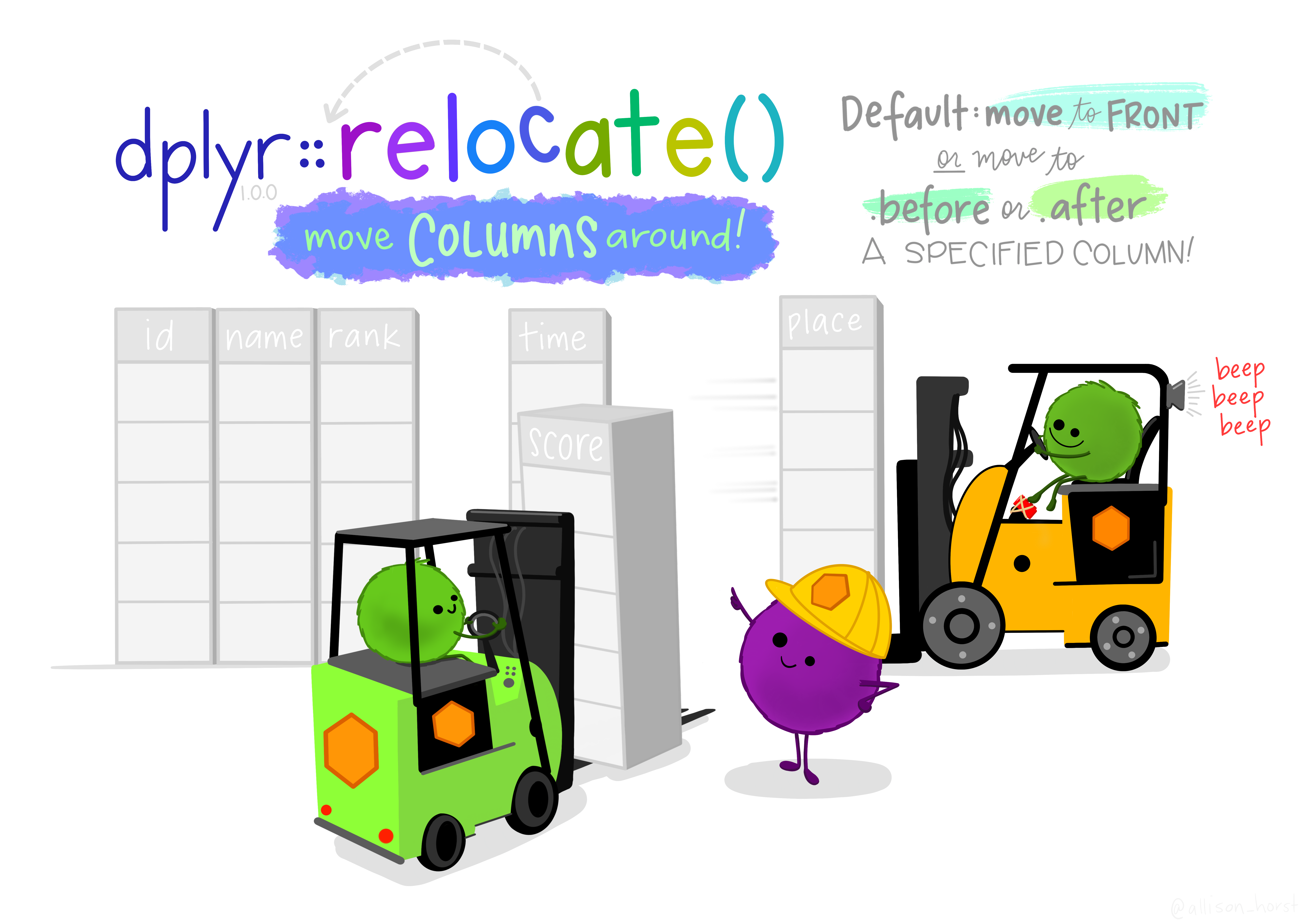
22.4.1 Rearranging Columns
Another handy dplyr function is relocate; while you definitely can do this operation in many, many different ways, it may be simpler to do it using relocate. But, I’m covering relocate here mostly because it also comes with this amazing cartoon illustration.
# Move flight specific info to the front
data(flights, package = "nycflights13")
relocate(flights, carrier:dest, everything())
## # A tibble: 336,776 × 19
##    carrier flight tailnum origin dest   year month   day dep_time sched_dep_time
##    <chr>    <int> <chr>   <chr>  <chr> <int> <int> <int>    <int>          <int>
##  1 UA        1545 N14228  EWR    IAH    2013     1     1      517            515
##  2 UA        1714 N24211  LGA    IAH    2013     1     1      533            529
##  3 AA        1141 N619AA  JFK    MIA    2013     1     1      542            540
##  4 B6         725 N804JB  JFK    BQN    2013     1     1      544            545
##  5 DL         461 N668DN  LGA    ATL    2013     1     1      554            600
##  6 UA        1696 N39463  EWR    ORD    2013     1     1      554            558
##  7 B6         507 N516JB  EWR    FLL    2013     1     1      555            600
##  8 EV        5708 N829AS  LGA    IAD    2013     1     1      557            600
##  9 B6          79 N593JB  JFK    MCO    2013     1     1      557            600
## 10 AA         301 N3ALAA  LGA    ORD    2013     1     1      558            600
## # ℹ 336,766 more rows
## # ℹ 9 more variables: dep_delay <dbl>, arr_time <int>, sched_arr_time <int>,
## #   arr_delay <dbl>, air_time <dbl>, distance <dbl>, hour <dbl>, minute <dbl>,
## #   time_hour <dttm>

# move numeric variables to the front
flights %>% relocate(where(is.numeric))
## # A tibble: 336,776 × 19
##     year month   day dep_time sched_dep_time dep_delay arr_time sched_arr_time
##    <int> <int> <int>    <int>          <int>     <dbl>    <int>          <int>
##  1  2013     1     1      517            515         2      830            819
##  2  2013     1     1      533            529         4      850            830
##  3  2013     1     1      542            540         2      923            850
##  4  2013     1     1      544            545        -1     1004           1022
##  5  2013     1     1      554            600        -6      812            837
##  6  2013     1     1      554            558        -4      740            728
##  7  2013     1     1      555            600        -5      913            854
##  8  2013     1     1      557            600        -3      709            723
##  9  2013     1     1      557            600        -3      838            846
## 10  2013     1     1      558            600        -2      753            745
## # ℹ 336,766 more rows
## # ℹ 11 more variables: arr_delay <dbl>, flight <int>, air_time <dbl>,
## #   distance <dbl>, hour <dbl>, minute <dbl>, carrier <chr>, tailnum <chr>,
## #   origin <chr>, dest <chr>, time_hour <dttm>
There are similar ways to rearrange columns in pandas, but they are a bit harder to work with - you have to specify the column names (in some way) and then perform the operation yourself.
import numpy as np
cols = list(flights.columns.values) # get column names
# Move flight specific info to the front
flightcols = ['carrier', 'flight', 'tailnum', 'origin', 'dest']
flights[flightcols + list(flights.drop(flightcols, axis = 1))]
## carrier flight tailnum ... hour minute time_hour
## 0 UA 1545 N14228 ... 5 15 2013-01-01T10:00:00Z
## 1 UA 1714 N24211 ... 5 29 2013-01-01T10:00:00Z
## 2 AA 1141 N619AA ... 5 40 2013-01-01T10:00:00Z
## 3 B6 725 N804JB ... 5 45 2013-01-01T10:00:00Z
## 4 DL 461 N668DN ... 6 0 2013-01-01T11:00:00Z
## ... ... ... ... ... ... ... ...
## 336771 9E 3393 NaN ... 14 55 2013-09-30T18:00:00Z
## 336772 9E 3525 NaN ... 22 0 2013-10-01T02:00:00Z
## 336773 MQ 3461 N535MQ ... 12 10 2013-09-30T16:00:00Z
## 336774 MQ 3572 N511MQ ... 11 59 2013-09-30T15:00:00Z
## 336775 MQ 3531 N839MQ ... 8 40 2013-09-30T12:00:00Z
##
## [336776 rows x 19 columns]
# move numeric variables to the front
numcols = list(flights.select_dtypes(include = np.number).columns.values)
flights[numcols + list(flights.drop(numcols, axis = 1))]
## year month day dep_time ... tailnum origin dest time_hour
## 0 2013 1 1 517.0 ... N14228 EWR IAH 2013-01-01T10:00:00Z
## 1 2013 1 1 533.0 ... N24211 LGA IAH 2013-01-01T10:00:00Z
## 2 2013 1 1 542.0 ... N619AA JFK MIA 2013-01-01T10:00:00Z
## 3 2013 1 1 544.0 ... N804JB JFK BQN 2013-01-01T10:00:00Z
## 4 2013 1 1 554.0 ... N668DN LGA ATL 2013-01-01T11:00:00Z
## ... ... ... ... ... ... ... ... ... ...
## 336771 2013 9 30 NaN ... NaN JFK DCA 2013-09-30T18:00:00Z
## 336772 2013 9 30 NaN ... NaN LGA SYR 2013-10-01T02:00:00Z
## 336773 2013 9 30 NaN ... N535MQ LGA BNA 2013-09-30T16:00:00Z
## 336774 2013 9 30 NaN ... N511MQ LGA CLE 2013-09-30T15:00:00Z
## 336775 2013 9 30 NaN ... N839MQ LGA RDU 2013-09-30T12:00:00Z
##
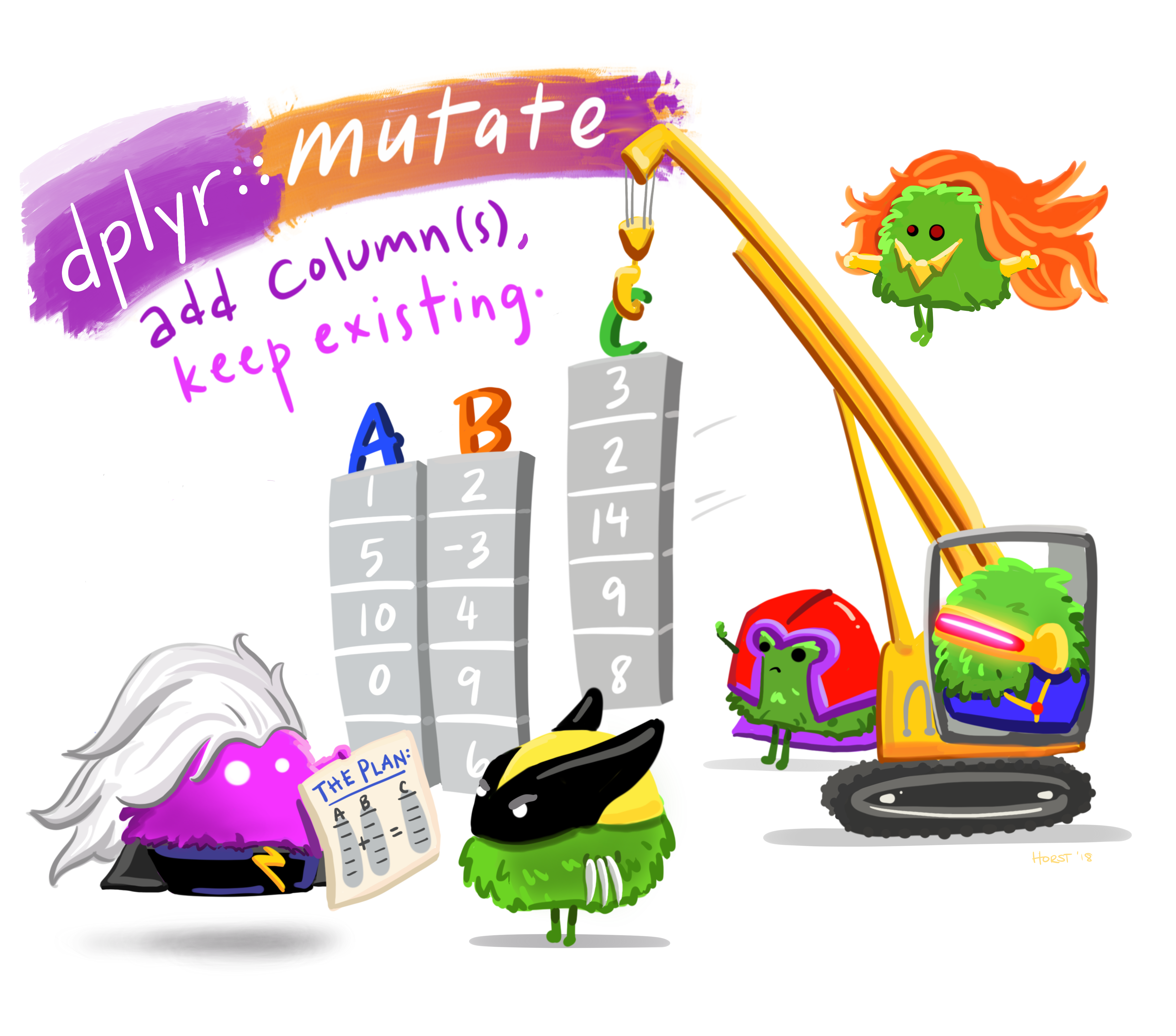
## [336776 rows x 19 columns]22.5 Mutate: Add and transform variables
Up to this point, we’ve been primarily focusing on how to decrease the dimensionality of our dataset in various ways. But frequently, we also need to add columns for derived measures (e.g. BMI from weight and height information), change units, and replace missing or erroneous observations. The tidyverse verb for this is mutate, but in base R and python, we’ll simply use assignment to add columns to our data frames.
We’ll use the Pokemon data to demonstrate. Some Pokemon have a single “type”, which is usually elemental, such as Water, Ice, Fire, etc., but others have two. Let’s add a column that indicates how many types a pokemon has.
poke <- read_csv("https://github.com/srvanderplas/datasets/raw/main/clean/pokemon_gen_1-9.csv")

# This splits type_1,type_2 into two separate variables.
# Don't worry about the string processing (gsub) just now
# Focus on how variables are defined.
poke$type_1 <- gsub(",.*$", "", poke$type) # Replace anything after comma with ''
poke$type_2 <- gsub("^.*,", "", poke$type) # Use the 2nd type
poke$type_2[poke$type_1 == poke$type_2] <- NA # Type 2 only exists if not same as Type 1

poke$no_types <- 1 # set a default value
poke$no_types[grepl(",", poke$type)] <- 2 # set the value if there's not a comma in type

# This is a bit faster
poke$no_types <- ifelse(grepl(",", poke$type), 2, 1)

# Sanity check
# This checks number of types vs. value of type_2
# If type 2 is NA, then number of types should be 1
t(table(poke$type_2, poke$no_types, useNA = 'ifany'))
##
##     Bug Dark Dragon Electric Fairy Fighting Fire Flying Ghost Grass Ground Ice
##   1   0    0      0        0     0        0    0      0     0     0      0   0
##   2   9   40     49       17    47       47   31    157    57    50     57  36
##
##     Normal Poison Psychic Rock Steel Water <NA>
##   1      0      0       0    0     0     0  673
##   2     24     51      61   23    55    42    0
Notice that we had to type the name of the dataset at least 3 times to perform the operation we were looking for. I could reduce that to 2x with the ifelse function, but it’s still a lot of typing.
poke <- read_csv("https://github.com/srvanderplas/datasets/raw/main/clean/pokemon_gen_1-9.csv")

poke <- poke %>%
  # This splits type into type_1,type_2 : two separate variables.
  # Don't worry about the string processing (str_extract) just now
  # Focus on how variables are defined:
  #   we use a function on the type column
  #   within the mutate statement.
  mutate(type_1 = str_extract(type, "^(.*),", group = 1),
         type_2 = str_extract(type, "(.*),(.*)", group = 2)) %>%
  mutate(no_types = if_else(is.na(type_2), 1, 2))
## Error in `mutate()` at dplyr/R/mutate.R:146:3:
## ℹ In argument: `type_1 = str_extract(type, "^(.*),", group = 1)`.
## Caused by error in `str_extract()`:
## ! could not find function "str_extract"

select(poke, type_2, no_types) %>% table(useNA = 'ifany') %>% t()
## Error in `select()`:
## ! Can't select columns that don't exist.
## ✖ Column `type_2` doesn't exist.
The last 2 rows are just to organize the output - we keep only the two variables we’re working with, and get a crosstab.
In python, this type of variable operation (replacing one value with another) can be most easily done with the replace function, which takes arguments (thing_to_replace, value_to_replace_with).
import pandas as pd
poke = pd.read_csv("https://github.com/srvanderplas/datasets/raw/main/clean/pokemon_gen_1-9.csv")

# This splits type into two columns, type_1 and type_2, based on ","
poke[["type_1", "type_2"]] = poke["type"].apply(lambda x: pd.Series(str(x).split(",")))

# This defines number of types
poke["no_types"] = 1 # default value
poke.loc[~poke.type_2.isna(), "no_types"] = 2 # change those with a defined type 2


poke.groupby(["no_types", "type_2"], dropna=False).size()
## no_types  type_2
## 1         NaN         673
## 2         Bug           9
##           Dark         40
##           Dragon       49
##           Electric     17
##           Fairy        47
##           Fighting     47
##           Fire         31
##           Flying      157
##           Ghost        57
##           Grass        50
##           Ground       57
##           Ice          36
##           Normal       24
##           Poison       51
##           Psychic      61
##           Rock         23
##           Steel        55
##           Water        42
## dtype: int64
# When type_2 is NaN, no_types is 1
# When type_2 is defined, no_types is 2
Another function that may be useful is the assign function, which can be used to create new variables if you don’t want to use the ["new_col"] notation. In some circumstances, .assign(var = ...) is a bit easier to work with because Python distinguishes between modifications to data and making a copy of the entire data frame (which is something I’d like to not get into right now for simplicity’s sake).
The learning curve here isn’t actually knowing how to assign new variables (though that’s important). The challenge comes when you want to do something new and have to figure out how to e.g. use find and replace in a string, or work with dates and times, or recode variables.
Mutate and new challenges
I’m not going to be able to teach you how to handle every mutate statement task you’ll come across (people invent new ways to screw up data all the time!) but my goal is instead to teach you how to read documentation, google things intelligently, and to understand what you’re reading enough to actually implement it. This is something that comes with practice (and lots of googling, stack overflow searches, etc.).
Google and StackOverflow are very common and important programming skills!


In this textbook, the examples will expose you to solutions to common problems (or require that you do some basic reading yourself); unfortunately, there are too many common problems for us to work through line-by-line.
Part of the goal of this textbook is to help you learn how to read through a package description and evaluate whether the package will do what you want. We’re going to try to build some of those skills starting now. It would be relatively easy to teach you how to do a set list of tasks, but you’ll be better statisticians and programmers if you learn the skills to solve niche problems on your own.

Note
Here is a quick table of places to look in R and python to solve some of the more common problems.
| Problem | R | Python |
|---|---|---|
| Dates and Times |
lubridate package (esp. ymd_hms() and variants, decimal_date(), and other convenience functions) |
pandas has some date time support by default; see the datetime module for more functionality. |
| String manipulation |
stringr package |
Quick Tips [5], Whirlwind Tour of Python chapter [6] |
22.6 Summarize
The next verb is one that we’ve already implicitly seen in action: summarize takes a data frame with potentially many rows of data and reduces it down to one row of data using some function. You have used it to get single-row summaries of vectorized data in R, and we’ve used e.g. group_by + count in Python to perform certain tasks as well.
Here (in a trivial example), I compute the overall average HP of a Pokemon in each generation, as well as the average number of characters in their name. Admittedly, that last computation is a bit silly, but it’s mostly for demonstration purposes.
In python, instead of a summarize function, there are a number of shorthand functions that we often use to summarize things, such as mean. You can also build custom summary functions [7], or use the agg() function to define multiple summary variables. agg() will even let you use different summary functions for each variable, just like summarize.
import pandas as pd

poke = pd.read_csv("https://github.com/srvanderplas/datasets/raw/main/clean/pokemon_gen_1-9.csv")

poke = poke.assign(name_length = poke.name.str.len())
poke[['hp', 'name_length']].mean()
## hp             71.178244
## name_length     7.545216
## dtype: float64
poke[['hp', 'name_length']].agg(['mean', 'min'])
##              hp  name_length
## mean  71.178244     7.545216
## min    1.000000     3.000000
poke[['pokedex_no', 'hp', 'name_length']].agg({'pokedex_no':'nunique', 'hp':'mean', 'name_length':'mean'})
## pokedex_no     1008.000000
## hp               71.178244
## name_length       7.545216
## dtype: float64
The real power of summarize, though, is in combination with Group By. We’ll see more summarize examples, but it’s easier to make good examples when you have all the tools - it’s hard to demonstrate how to use a hammer if you don’t also have a nail.
22.7 Group By + (?) = Power!
Frequently, we have data that is more specific than the data we need - for instance, I may have observations of the temperature at 15-minute intervals, but I might want to record the daily high and low value. To do this, I need to
- split my dataset into smaller datasets - one for each day
- compute summary values for each smaller dataset
- put my summarized data back together into a single dataset
This is known as the split-apply-combine [9] or sometimes, map-reduce [10] strategy (though map-reduce is usually on specifically large datasets and performed in parallel).
In tidy parlance, group_by is the verb that accomplishes the first task. summarize accomplishes the second task and implicitly accomplishes the third as well.

poke <- read_csv("https://github.com/srvanderplas/datasets/raw/main/clean/pokemon_gen_1-9.csv")
poke %>%
  mutate(name_chr = nchar(name)) %>%
  group_by(gen) %>%
  summarize(n = length(unique(pokedex_no)), hp = mean(hp), name_chr = mean(name_chr))
## # A tibble: 9 × 4
##     gen     n    hp name_chr
##   <dbl> <int> <dbl>    <dbl>
## 1     1   151  65.3     7.23
## 2     2   100  71.0     7.36
## 3     3   135  65.8     7.16
## 4     4   107  69.4     6.85
## 5     5   156  75.8     7.77
## 6     6    72  72.9     7.47
## 7     7    88  73.2     8.04
## 8     8    96  77.9     8.01
## 9     9   103  75.8     8.66
import pandas as pd
poke = pd.read_csv("https://github.com/srvanderplas/datasets/raw/main/clean/pokemon_gen_1-9.csv")
poke = poke.assign(name_length = poke.name.str.len())
poke.groupby('gen')[['hp', 'name_length']].mean()
## hp name_length
## gen
## 1 65.333333 7.231579
## 2 71.024194 7.362903
## 3 65.777202 7.160622
## 4 69.382022 6.853933
## 5 75.827004 7.767932
## 6 72.882353 7.470588
## 7 73.233083 8.037594
## 8 77.940299 8.014925
## 9 75.756098 8.658537
poke.groupby('gen')[['hp', 'name_length']].agg(['mean', 'min'])
## hp name_length
## mean min mean min
## gen
## 1 65.333333 10 7.231579 3
## 2 71.024194 20 7.362903 4
## 3 65.777202 1 7.160622 4
## 4 69.382022 20 6.853933 4
## 5 75.827004 30 7.767932 4
## 6 72.882353 38 7.470588 5
## 7 73.233083 25 8.037594 6
## 8 77.940299 25 8.014925 4
## 9 75.756098 10 8.658537 5
poke.groupby('gen')[['pokedex_no', 'hp', 'name_length']].agg({'pokedex_no':'nunique', 'hp':'mean', 'name_length':'mean'})
## pokedex_no hp name_length
## gen
## 1 151 65.333333 7.231579
## 2 100 71.024194 7.362903
## 3 135 65.777202 7.160622
## 4 107 69.382022 6.853933
## 5 156 75.827004 7.767932
## 6 72 72.882353 7.470588
## 7 88 73.233083 8.037594
## 8 96 77.940299 8.014925
## 9 103 75.756098 8.658537When you group_by a variable, your result carries this grouping with it. In R, summarize will remove one layer of grouping (by default), but if you ever want to return to a completely ungrouped data set, you should use the ungroup() command. In Python, you should consider using reset_index or grouped_thing.obj() to access the original information[11].
Storms Example
Let’s try a non-trivial example, using the storms dataset that is part of the dplyr package.
library(dplyr)
library(lubridate) # for the make_datetime() function
data(storms)
storms
## # A tibble: 19,537 × 13
##    name   year month   day  hour   lat  long status      category  wind pressure
##    <chr> <dbl> <dbl> <int> <dbl> <dbl> <dbl> <fct>          <dbl> <int>    <int>
##  1 Amy    1975     6    27     0  27.5 -79   tropical d…       NA    25     1013
##  2 Amy    1975     6    27     6  28.5 -79   tropical d…       NA    25     1013
##  3 Amy    1975     6    27    12  29.5 -79   tropical d…       NA    25     1013
##  4 Amy    1975     6    27    18  30.5 -79   tropical d…       NA    25     1013
##  5 Amy    1975     6    28     0  31.5 -78.8 tropical d…       NA    25     1012
##  6 Amy    1975     6    28     6  32.4 -78.7 tropical d…       NA    25     1012
##  7 Amy    1975     6    28    12  33.3 -78   tropical d…       NA    25     1011
##  8 Amy    1975     6    28    18  34   -77   tropical d…       NA    30     1006
##  9 Amy    1975     6    29     0  34.4 -75.8 tropical s…       NA    35     1004
## 10 Amy    1975     6    29     6  34   -74.8 tropical s…       NA    40     1002
## # ℹ 19,527 more rows
## # ℹ 2 more variables: tropicalstorm_force_diameter <int>,
## #   hurricane_force_diameter <int>

storms <- storms %>%
  # Construct a time variable that behaves like a number but is formatted as a date
  mutate(time = make_datetime(year, month, day, hour))
import pandas as pd
import numpy as np
storms = pd.read_csv("https://raw.githubusercontent.com/srvanderplas/datasets/main/clean/storms.csv", on_bad_lines='skip')
# Construct a time variable that behaves like a number but is formatted as a date
storms = storms.assign(time = pd.to_datetime(storms[["year", "month", "day", "hour"]]))
# Remove month/day/hour
# (keep year for ID purposes, names are reused)
storms = storms.drop(["month", "day", "hour"], axis = 1)We have named storms, observation time, storm location, status, wind, pressure, and diameter (for tropical storms and hurricanes).
One thing we might want to know is at what point each storm was the strongest. Let’s define strongest in the following way:
- The points where the storm is at its lowest atmospheric pressure (generally, the lower the atmospheric pressure, the more trouble a tropical disturbance will cause).
- If there’s a tie, we might want to know when the maximum wind speed occurred.
- If that still doesn’t get us a single row for each observation, lets just pick out the status and category (these are determined by wind speed, so they should be the same if maximum wind speed is the same) and compute the average time where this occurred.
Let’s start by translating these criteria into basic operations. I’ll use dplyr function names here, but I’ll also specify what I mean when there’s a conflict (e.g. filter in dplyr means something different than filter in python).
Initial attempt:
-
For each storm (
group_by), - we need the point where the storm has lowest atmospheric pressure. (
filter- pick the row with the lowest pressure).
Then we read the next part: “If there is a tie, pick the maximum wind speed.”
group_by-
arrangeby ascending pressure and descending wind speed -
filter- pick the row(s) which have the lowest pressure and highest wind speed
Then, we read the final condition: if there is still a tie, pick the status and category and compute the average time.
group_by-
arrangeby ascending pressure and descending wind speed (this is optional if we write our filter in a particular way) -
filter- pick the row(s) which have the lowest pressure and highest wind speed -
summarize- compute the average time and category (if there are multiple rows)
Let’s write the code, now that we have the order of operations straight!
max_power_storm <- storms %>%
  # Storm names can be reused, so we need to have year to be sure it's the same instance
  group_by(name, year) %>%
  filter(pressure == min(pressure, na.rm = T)) %>%
  filter(wind == max(wind, na.rm = T)) %>%
  summarize(pressure = mean(pressure),
            wind = mean(wind),
            category = unique(category),
            status = unique(status),
            time = mean(time)) %>%
  arrange(time) %>%
  ungroup()
max_power_storm
## # A tibble: 665 × 7
##    name      year pressure  wind category status         time
##    <chr>    <dbl>    <dbl> <dbl>    <dbl> <fct>          <dttm>
##  1 Amy       1975      981    60       NA tropical storm 1975-07-02 12:00:00
##  2 Blanche   1975      980    75        1 hurricane      1975-07-28 00:00:00
##  3 Caroline  1975      963   100        3 hurricane      1975-08-31 06:00:00
##  4 Doris     1975      965    95        2 hurricane      1975-09-02 21:00:00
##  5 Eloise    1975      955   110        3 hurricane      1975-09-23 12:00:00
##  6 Faye      1975      977    75        1 hurricane      1975-09-28 18:00:00
##  7 Gladys    1975      939   120        4 hurricane      1975-10-02 15:00:00
##  8 Hallie    1975     1002    45       NA tropical storm 1975-10-27 03:00:00
##  9 Belle     1976      957   105        3 hurricane      1976-08-09 00:00:00
## 10 Dottie    1976      996    45       NA tropical storm 1976-08-20 06:00:00
## # ℹ 655 more rows
grouped_storms = storms.groupby(["name", "year"])
grouped_storm_sum = grouped_storms.agg({
"pressure": lambda x: x.min()
}).reindex()
# This gets all the information from storms
# corresponding to name/year/max pressure
max_power_storm = grouped_storm_sum.merge(storms, on = ["name", "year", "pressure"])
max_power_storm = max_power_storm.groupby(["name", "year"]).agg({
"pressure": "min",
"wind": "max",
"category": "mean",
"status": "unique",
"time": "mean"
})If we want to see a visual summary, we could plot a histogram of the minimum pressure of each storm.
library(ggplot2)
ggplot(max_power_storm, aes(x = pressure)) + geom_histogram()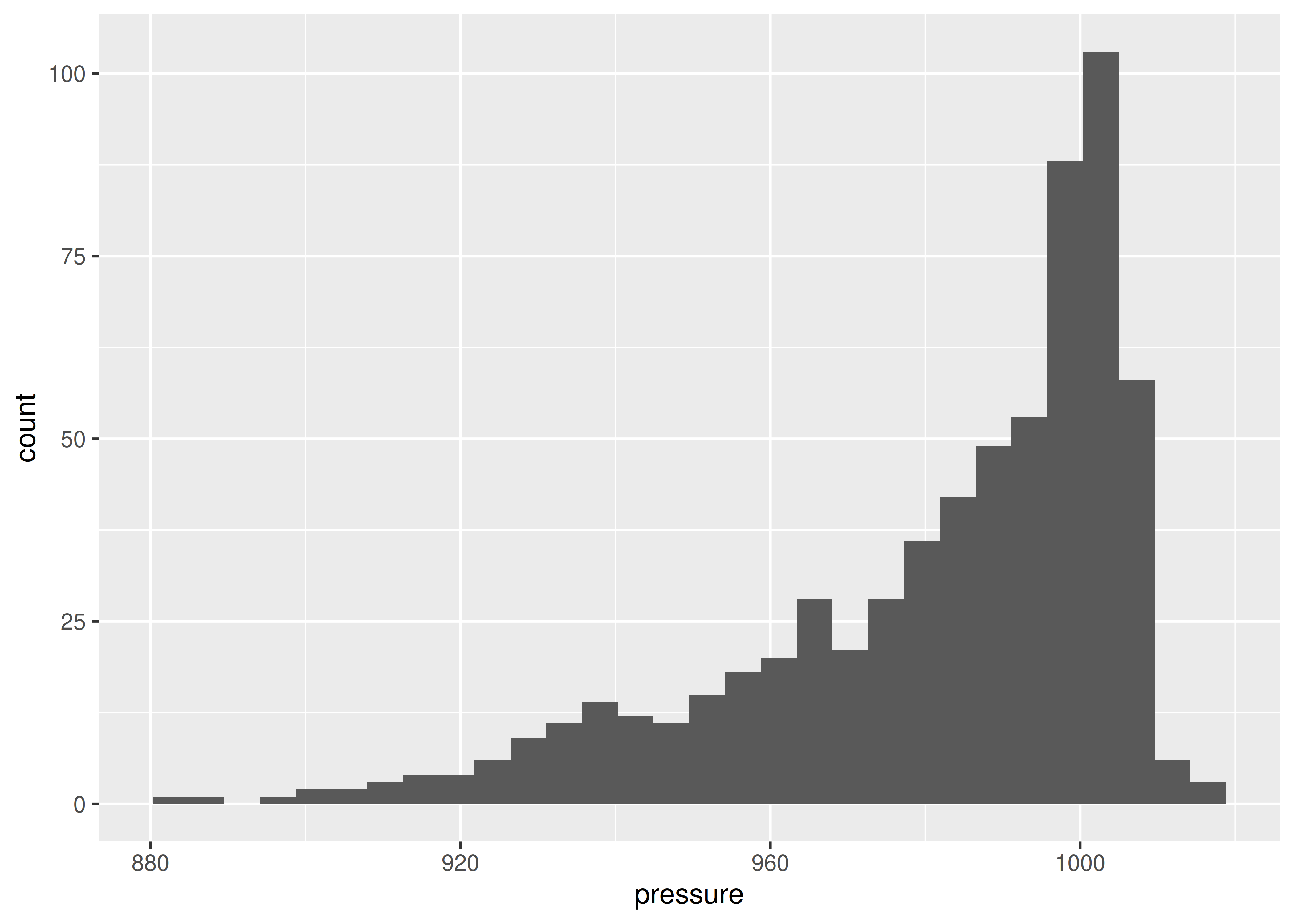
from plotnine import *

ggplot(max_power_storm, aes(x = "pressure")) + geom_histogram(bins=30)
## <plotnine.ggplot.ggplot object at 0x7fb3eae75b10>
We could also look to see whether there has been any change over time in pressure.
ggplot(max_power_storm, aes(x = time, y = pressure)) + geom_point()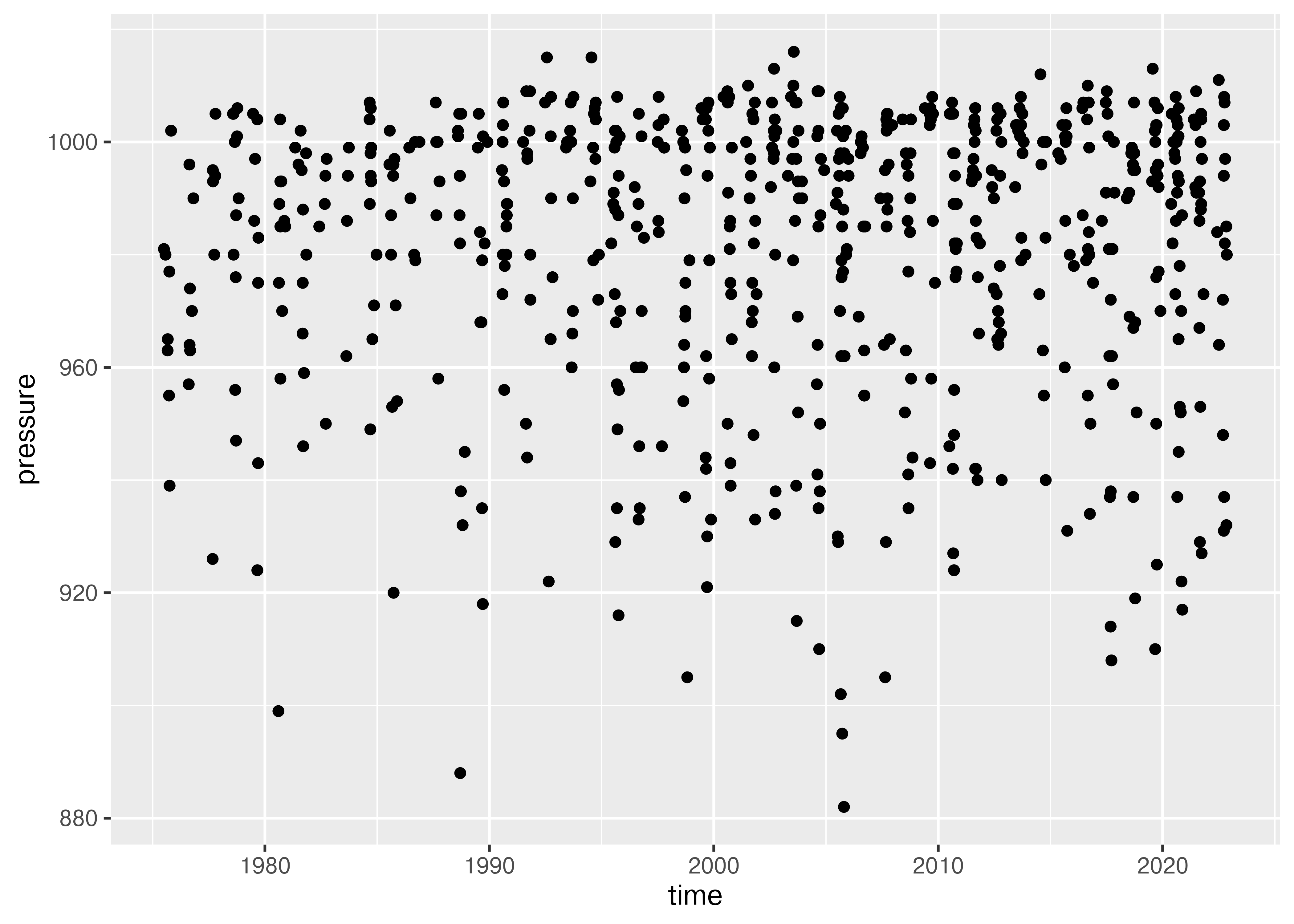
ggplot(max_power_storm, aes(x = "time", y = "pressure")) + geom_point()
## <plotnine.ggplot.ggplot object at 0x7fb3ea855810>
It seems to me that there are fewer high-pressure storms before 1990 or so, which may be due to the fact that some weak storms may not have been observed or recorded prior to widespread radar coverage in the Atlantic.
Another interesting way to look at this data would be to examine the duration of time a storm existed, as a function of its maximum category. Do stronger storms exist for a longer period of time?
storm_strength_duration <- storms %>%
  group_by(name, year) %>%
  summarize(duration = difftime(max(time), min(time), units = "days"),
            max_strength = max(category)) %>%
  ungroup() %>%
  arrange(desc(max_strength))

storm_strength_duration %>%
  ggplot(aes(x = max_strength, y = duration)) + geom_boxplot()
## Error in `geom_boxplot()`:
## ! Problem while computing stat.
## ℹ Error occurred in the 1st layer.
## Caused by error in `if (...) NULL`:
## ! missing value where TRUE/FALSE needed
storm_strength_duration = storms.groupby(["name", "year"]).agg(duration = ("time", lambda x: max(x) - min(x)),max_strength = ("category", "max"))
ggplot(aes(x = "factor(max_strength)", y = "duration"), data = storm_strength_duration) + geom_boxplot()
## TypeError: ggplot.__init__() got multiple values for argument 'data'You don’t need to know how to create these plots yet, but I find it much easier to look at the chart and answer the question I started out with.
We could also look to see how a storm’s diameter evolves over time, from when the storm is first identified (group_by + mutate)
Diameter measurements don’t exist for all storms, and they appear to measure the diameter of the wind field - that is, the region where the winds are hurricane or tropical storm force. (?storms documents the dataset and its variables).
Note the use of as.numeric(as.character(max(category))) to get the maximum (ordinal categorical) strength and convert that into something numeric that can be plotted.
storm_evolution <- storms %>%
  filter(!is.na(hurricane_force_diameter)) %>%
  group_by(name, year) %>%
  mutate(time_since_start = difftime(time, min(time), units = "days")) %>%
  ungroup()

ggplot(storm_evolution,
       aes(x = time_since_start, y = hurricane_force_diameter,
           group = name)) + geom_line(alpha = .2) +
  facet_wrap(~year, scales = "free_y")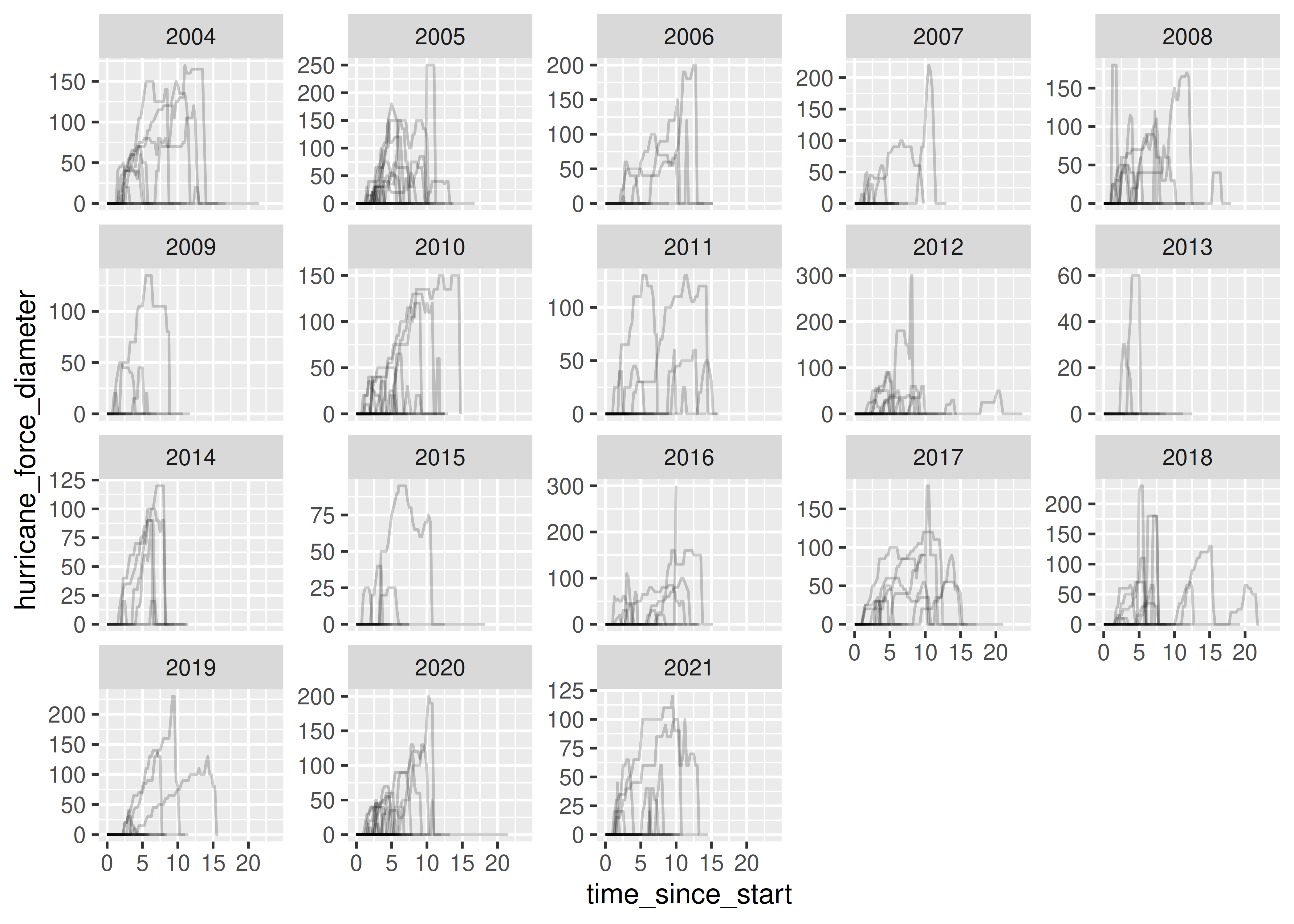
storm_evolution = storms.loc[storms.hurricane_force_diameter.notnull(),:]

storm_evolution = storm_evolution.assign(age = storm_evolution.groupby(["name", "year"], group_keys = False).apply(lambda x: x.time - x.time.min()))

(ggplot(storm_evolution,
       aes(x = "age", y = "hurricane_force_diameter",
           group = "name")) + geom_line(alpha = .2) +
  facet_wrap("year", scales = "free_y"))
## <plotnine.ggplot.ggplot object at 0x7fb3eb316350>
For this plot, I’ve added facet_wrap(~year) to produce sub-plots for each year. This helps us to be able to see some individuality, because otherwise there are far too many storms.
It seems that the vast majority of storms have a single bout of hurricane force winds (which either decreases or just terminates near the peak, presumably when the storm hits land and rapidly disintegrates). However, there are a few interesting exceptions - my favorite is in 2008 - the longest-lasting storm seems to have several local peaks in wind field diameter. If we want, we can examine that further by plotting it separately.
storm_evolution %>%
  filter(year == 2008) %>%
  arrange(desc(time_since_start))
## # A tibble: 548 × 15
##    name    year month   day  hour   lat  long status     category  wind pressure
##    <chr>  <dbl> <dbl> <int> <dbl> <dbl> <dbl> <fct>         <dbl> <int>    <int>
##  1 Bertha  2008     7    21     6  58.5 -27   extratrop…       NA    45      990
##  2 Bertha  2008     7    21     0  55.1 -31   extratrop…       NA    50      990
##  3 Bertha  2008     7    20    18  53   -34   extratrop…       NA    55      990
##  4 Bertha  2008     7    20    12  50   -37   extratrop…       NA    60      985
##  5 Bertha  2008     7    20     6  47.6 -40   tropical …       NA    60      985
##  6 Bertha  2008     7    20     0  45.3 -42.4 tropical …       NA    60      990
##  7 Bertha  2008     7    19    18  43.7 -44.3 hurricane         1    65      989
##  8 Bertha  2008     7    19    12  42.1 -46.3 hurricane         1    65      989
##  9 Bertha  2008     7    19     6  40.4 -48   hurricane         1    65      989
## 10 Bertha  2008     7    19     0  38.6 -49.7 hurricane         1    65      989
## # ℹ 538 more rows
## # ℹ 4 more variables: tropicalstorm_force_diameter <int>,
## #   hurricane_force_diameter <int>, time <dttm>, time_since_start <drtn>

storm_evolution %>% filter(name == "Ike") %>%
  ggplot(aes(x = time, y = hurricane_force_diameter, color = category)) + geom_point()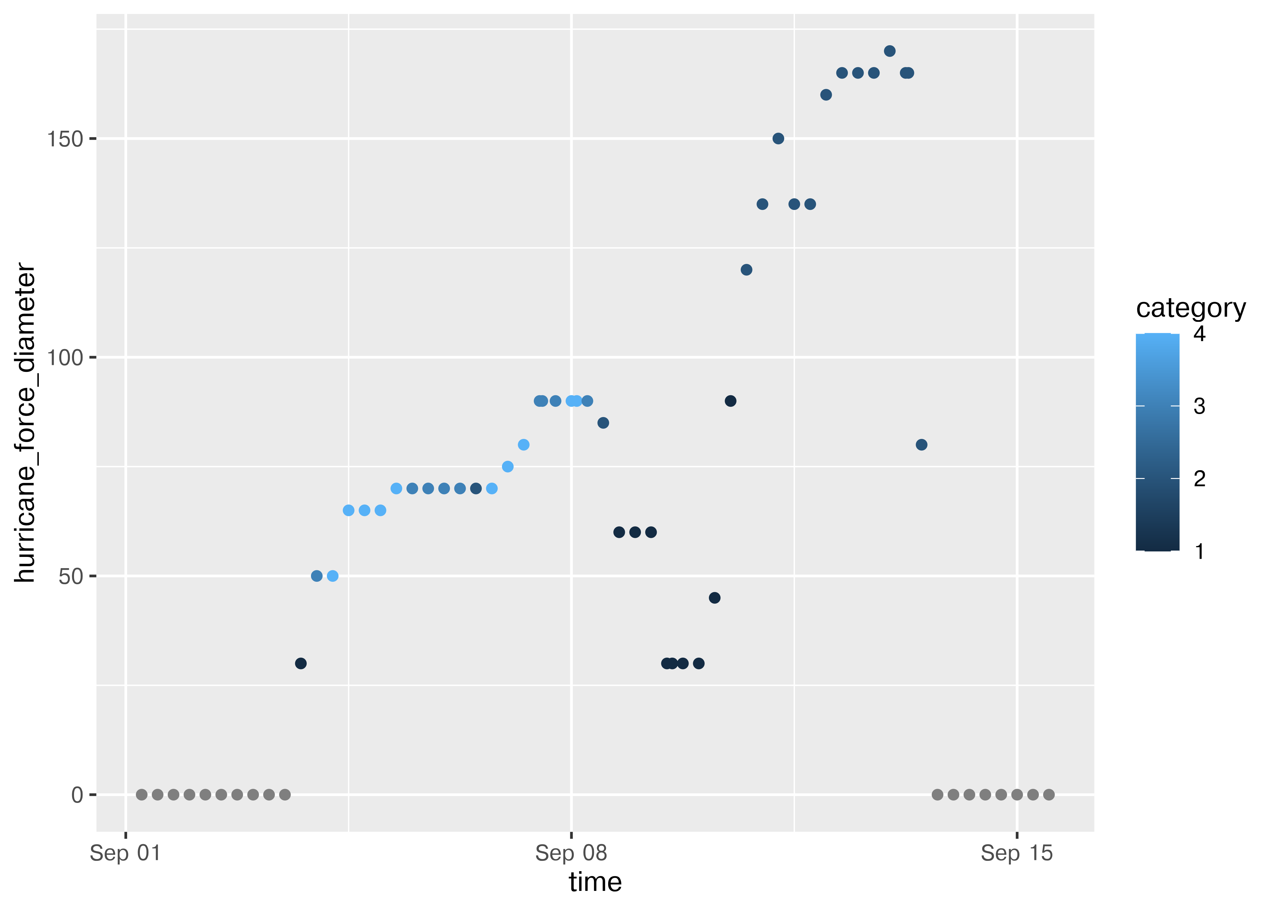
storm_evolution.query("year==2008").sort_values(['age'], ascending = False).head()
##      name  year  ...                time              age
## 8000  Ike  2008  ... 2008-09-14 06:00:00 13 days 00:00:00
## 7999  Ike  2008  ... 2008-09-14 00:00:00 12 days 18:00:00
## 7998  Ike  2008  ... 2008-09-13 18:00:00 12 days 12:00:00
## 7997  Ike  2008  ... 2008-09-13 12:00:00 12 days 06:00:00
## 7996  Ike  2008  ... 2008-09-13 07:00:00 12 days 01:00:00
##
## [5 rows x 12 columns]

(ggplot(
  storm_evolution.query("year==2008 & name=='Ike'"),
  aes(x = "time", y = "hurricane_force_diameter", color = "category")) +
  geom_point())
## <plotnine.ggplot.ggplot object at 0x7fb3ea6dfb10>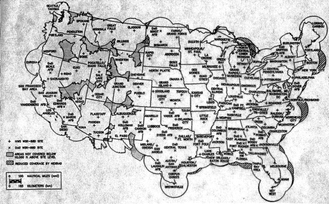
22.8 Summarizing Across Multiple Variables
Suppose we want to summarize the numerical columns of any storm which was a hurricane (over the entire period it was a hurricane). We don’t want to write out all of the summarize statements individually, so we use across() instead (in dplyr).
The dplyr package is filled with other handy functions for accomplishing common data-wrangling tasks. across() is particularly useful - it allows you to make a modification to several columns at the same time.
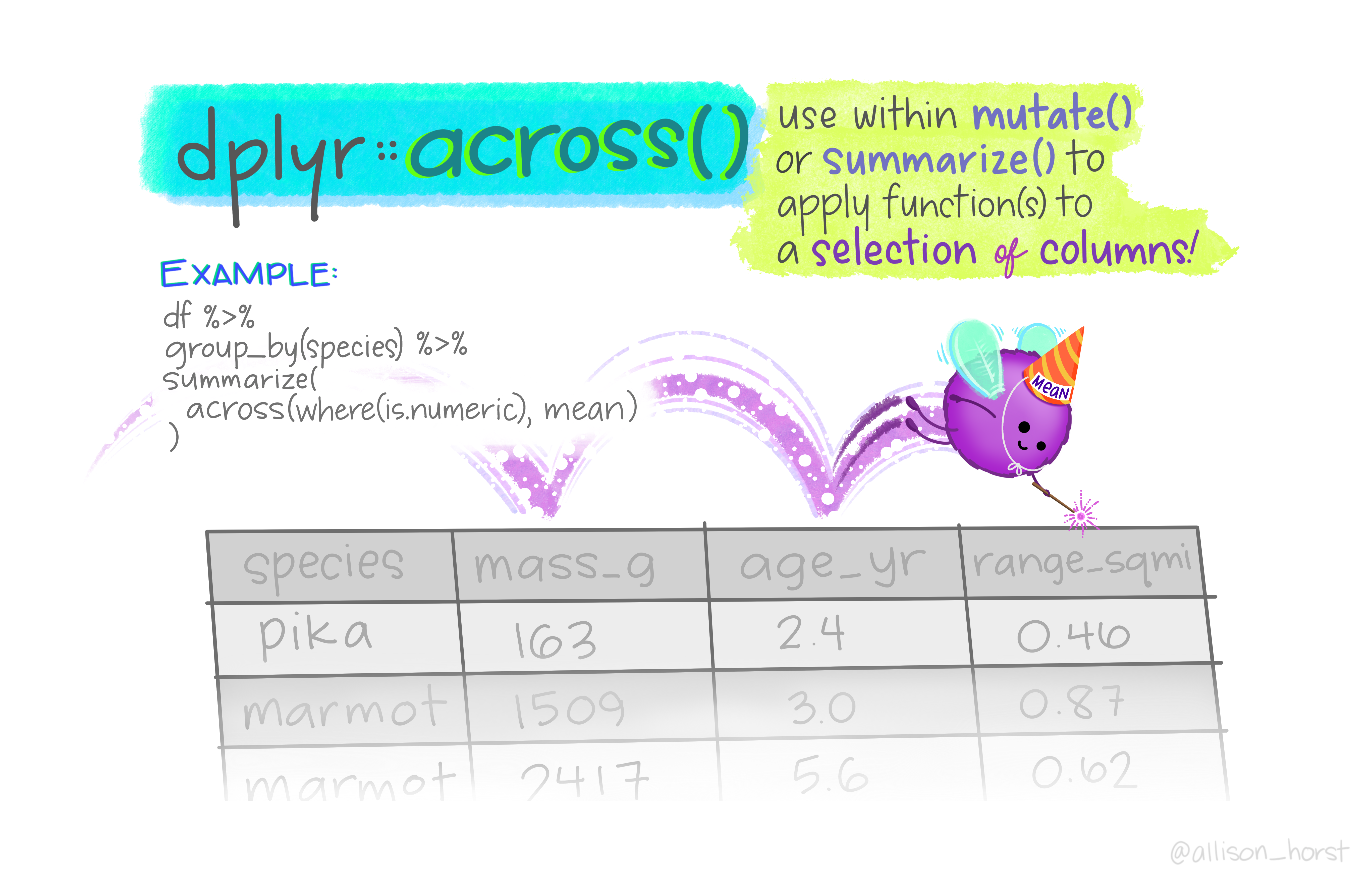
library(lubridate) # for the make_datetime() function
data(storms)

storms <- storms %>%
  # Construct a time variable that behaves like a number but is formatted as a date
  mutate(time = make_datetime(year, month, day, hour))

# Use across to get average of all numeric variables
avg_hurricane_intensity <- storms %>%
  filter(status == "hurricane") %>%
  group_by(name) %>%
  summarize(across(where(is.numeric), mean, na.rm = T), .groups = "drop")

avg_hurricane_intensity %>%
  select(name, year, month, wind, pressure, tropicalstorm_force_diameter, hurricane_force_diameter) %>%
  arrange(desc(wind)) %>%
  # get top 10
  filter(row_number() <= 10) %>%
knitr::kable() # Make into a pretty table| name | year | month | wind | pressure | tropicalstorm_force_diameter | hurricane_force_diameter |
|---|---|---|---|---|---|---|
| Allen | 1980 | 8.000000 | 122.9688 | 941.0312 | NaN | NaN |
| Irma | 2017 | 8.942308 | 118.8462 | 941.6154 | 249.4231 | 75.96154 |
| Andrew | 1992 | 8.000000 | 118.2609 | 946.6522 | NaN | NaN |
| Mitch | 1998 | 10.000000 | 115.9091 | 945.3182 | NaN | NaN |
| Rita | 2005 | 9.000000 | 114.7368 | 931.6316 | 265.2941 | 97.05882 |
| Isabel | 2003 | 9.000000 | 112.1875 | 946.5417 | NaN | NaN |
| Gilbert | 1988 | 9.000000 | 110.8929 | 945.4286 | NaN | NaN |
| Luis | 1995 | 8.928571 | 110.5952 | 948.6190 | NaN | NaN |
| Wilma | 2005 | 10.000000 | 110.3030 | 939.4242 | 349.8333 | 118.33333 |
| Matthew | 2016 | 9.880952 | 109.5238 | 952.1190 | 263.5714 | 62.02381 |
We can use python’s list comprehensions in combination with .agg to accomplish the same task as dplyr’s across function.
import pandas as pd
import numpy as np
storms = pd.read_csv("https://raw.githubusercontent.com/srvanderplas/datasets/main/clean/storms.csv")

# Construct a time variable that behaves like a number but is formatted as a date
storms = storms.assign(time = pd.to_datetime(storms[["year", "month", "day", "hour"]]))

# Remove year/month/day/hour
storms = storms.drop(["year", "month", "day", "hour"], axis = 1)

# Remove non-hurricane points
storms = storms.query("status == 'hurricane'")

# Get list of all remaining numeric variables
cols = storms.select_dtypes(include =[np.number]).columns.values
(storms.
set_index("name").
filter(cols).
groupby('name').
agg({col: 'mean' for col in cols}))
##                 lat  ...  hurricane_force_diameter
## name                 ...
## AL121991  38.850000  ...                       NaN
## Alberto   30.836735  ...                       NaN
## Alex      32.880769  ...                 48.461538
## Alicia    28.400000  ...                       NaN
## Allison   26.166667  ...                       NaN
## ...             ...  ...                       ...
## Teddy     25.793103  ...                103.448276
## Tomas     17.346154  ...                 24.230769
## Vince     34.100000  ...                 30.000000
## Wilma     22.327273  ...                118.333333
## Zeta      23.227273  ...                 29.545455
##
## [137 rows x 7 columns]
By default, pandas skips NaN values. If we want to be more clear, or want to pass another argument into the function, we can use what is called a lambda function - basically, a “dummy” function that has some arguments but not all of the arguments. Here, our lambda function is a function of x, and we calculate x.mean(skipna=True) for each x passed in (so, for each column).
# Get list of all remaining numeric variables
cols = storms.select_dtypes(include =[np.number]).columns.values
(storms.
set_index("name").
filter(cols).
groupby('name').
agg({col: lambda x: x.mean(skipna=True) for col in cols}))
##                 lat  ...  hurricane_force_diameter
## name                 ...
## AL121991  38.850000  ...                       NaN
## Alberto   30.836735  ...                       NaN
## Alex      32.880769  ...                 48.461538
## Alicia    28.400000  ...                       NaN
## Allison   26.166667  ...                       NaN
## ...             ...  ...                       ...
## Teddy     25.793103  ...                103.448276
## Tomas     17.346154  ...                 24.230769
## Vince     34.100000  ...                 30.000000
## Wilma     22.327273  ...                118.333333
## Zeta      23.227273  ...                 29.545455
##
## [137 rows x 7 columns]
22.9 Try it out - Data Cleaning
You can read about the gapminder project here.
The gapminder data used for this set of problems contains data from 142 countries on 5 continents. The filtered data in gapminder (in R) contain data about every 5 year period between 1952 and 2007, the country’s life expectancy at birth, population, and per capita GDP (in US $, inflation adjusted). In the gapminder_unfiltered table, however, things are a bit different. Some countries have yearly data, observations are missing, and some countries don’t have complete data. The gapminder package in python (install with pip install gapminder) is a port of the R package, but doesn’t contain the unfiltered data, so we’ll instead use a CSV export.
Read in the Data
if (!"gapminder" %in% installed.packages()) install.packages("gapminder")
library(gapminder)
gapminder_unfiltered
## # A tibble: 3,313 × 6
##    country     continent  year lifeExp      pop gdpPercap
##    <fct>       <fct>     <int>   <dbl>    <int>     <dbl>
##  1 Afghanistan Asia       1952    28.8  8425333      779.
##  2 Afghanistan Asia       1957    30.3  9240934      821.
##  3 Afghanistan Asia       1962    32.0 10267083      853.
##  4 Afghanistan Asia       1967    34.0 11537966      836.
##  5 Afghanistan Asia       1972    36.1 13079460      740.
##  6 Afghanistan Asia       1977    38.4 14880372      786.
##  7 Afghanistan Asia       1982    39.9 12881816      978.
##  8 Afghanistan Asia       1987    40.8 13867957      852.
##  9 Afghanistan Asia       1992    41.7 16317921      649.
## 10 Afghanistan Asia       1997    41.8 22227415      635.
## # ℹ 3,303 more rows
import pandas as pd
gapminder_unfiltered = pd.read_csv("https://raw.githubusercontent.com/srvanderplas/datasets/main/raw/gapminder_unfiltered.csv")
Task 1: How Bad is It?
Using your EDA skills, determine how bad the unfiltered data are. You may want to look for missing values, number of records, etc. Use query or filter to show any countries which have incomplete data. Describe, in words, what operations were necessary to get this information.
gapminder_unfiltered %>%
  group_by(country) %>%
  summarize(n = n(), missinglifeExp = sum(is.na(lifeExp)),
            missingpop = sum(is.na(pop)),
            missingGDP = sum(is.na(gdpPercap))) %>%
  filter(n != length(seq(1952, 2007, by = 5)))
## # A tibble: 83 × 5
##    country        n missinglifeExp missingpop missingGDP
##    <fct>      <int>          <int>      <int>      <int>
##  1 Armenia        4              0          0          0
##  2 Aruba          8              0          0          0
##  3 Australia     56              0          0          0
##  4 Austria       57              0          0          0
##  5 Azerbaijan     4              0          0          0
##  6 Bahamas       10              0          0          0
##  7 Barbados      10              0          0          0
##  8 Belarus       18              0          0          0
##  9 Belgium       57              0          0          0
## 10 Belize        11              0          0          0
## # ℹ 73 more rows
In order to determine what gaps were present in the gapminder dataset, I determined how many years of data were available for each country by grouping the dataset and counting the rows. There should be 12 years worth of data between 1952 and 2007; as a result, I displayed the countries which did not have exactly 12 years of data.
(
  gapminder_unfiltered.
  set_index("country").
  filter(["lifeExp", "pop", "gdpPercap"]).
  groupby("country").
  agg(lambda x: x.notnull().sum()).
  query("lifeExp != 12 | pop != 12 | gdpPercap != 12")
  )
##                       lifeExp  pop  gdpPercap
## country
## Armenia                     4    4          4
## Aruba                       8    8          8
## Australia                  56   56         56
## Austria                    57   57         57
## Azerbaijan                  4    4          4
## ...                       ...  ...        ...
## United Arab Emirates        8    8          8
## United Kingdom             13   13         13
## United States              57   57         57
## Uzbekistan                  4    4          4
## Vanuatu                     7    7          7
##
## [83 rows x 3 columns]
In order to determine what gaps were present in the gapminder dataset, I determined how many years of data were available for each country by grouping the dataset and counting the rows. There should be 12 years worth of data between 1952 and 2007; as a result, I displayed the countries which did not have exactly 12 years of data.
Task 2: Exclude any data which isn’t at 5-year increments
Start in 1952 (so 1952, 1957, 1962, …, 2007).
gapminder_unfiltered %>%
  filter(year %in% seq(1952, 2007, by = 5))
## # A tibble: 2,013 × 6
##    country     continent  year lifeExp      pop gdpPercap
##    <fct>       <fct>     <int>   <dbl>    <int>     <dbl>
##  1 Afghanistan Asia       1952    28.8  8425333      779.
##  2 Afghanistan Asia       1957    30.3  9240934      821.
##  3 Afghanistan Asia       1962    32.0 10267083      853.
##  4 Afghanistan Asia       1967    34.0 11537966      836.
##  5 Afghanistan Asia       1972    36.1 13079460      740.
##  6 Afghanistan Asia       1977    38.4 14880372      786.
##  7 Afghanistan Asia       1982    39.9 12881816      978.
##  8 Afghanistan Asia       1987    40.8 13867957      852.
##  9 Afghanistan Asia       1992    41.7 16317921      649.
## 10 Afghanistan Asia       1997    41.8 22227415      635.
## # ℹ 2,003 more rows
Reminder about python list comprehensions
Explanation of the query @ statement
years_to_keep = [i for i in range(1952, 2008, 5)]
gapminder_unfiltered.query("year in @years_to_keep")
##           country continent  year  lifeExp       pop   gdpPercap
## 0     Afghanistan      Asia  1952   28.801   8425333  779.445314
## 1     Afghanistan      Asia  1957   30.332   9240934  820.853030
## 2     Afghanistan      Asia  1962   31.997  10267083  853.100710
## 3     Afghanistan      Asia  1967   34.020  11537966  836.197138
## 4     Afghanistan      Asia  1972   36.088  13079460  739.981106
## ...           ...       ...   ...      ...       ...         ...
## 3308     Zimbabwe    Africa  1987   62.351   9216418  706.157306
## 3309     Zimbabwe    Africa  1992   60.377  10704340  693.420786
## 3310     Zimbabwe    Africa  1997   46.809  11404948  792.449960
## 3311     Zimbabwe    Africa  2002   39.989  11926563  672.038623
## 3312     Zimbabwe    Africa  2007   43.487  12311143  469.709298
##
## [2013 rows x 6 columns]
Task 3: Exclude any countries that don’t have a full set of observations
gapminder_unfiltered %>%
  filter(year %in% seq(1952, 2007, by = 5)) %>%
  group_by(country) %>%
  mutate(nobs = n()) %>% # Use mutate instead of summarize so that all rows stay
  filter(nobs == 12) %>%
  select(-nobs)
## # A tibble: 1,704 × 6
## # Groups:   country [142]
##    country     continent  year lifeExp      pop gdpPercap
##    <fct>       <fct>     <int>   <dbl>    <int>     <dbl>
##  1 Afghanistan Asia       1952    28.8  8425333      779.
##  2 Afghanistan Asia       1957    30.3  9240934      821.
##  3 Afghanistan Asia       1962    32.0 10267083      853.
##  4 Afghanistan Asia       1967    34.0 11537966      836.
##  5 Afghanistan Asia       1972    36.1 13079460      740.
##  6 Afghanistan Asia       1977    38.4 14880372      786.
##  7 Afghanistan Asia       1982    39.9 12881816      978.
##  8 Afghanistan Asia       1987    40.8 13867957      852.
##  9 Afghanistan Asia       1992    41.7 16317921      649.
## 10 Afghanistan Asia       1997    41.8 22227415      635.
## # ℹ 1,694 more rows
years_to_keep = [i for i in range(1952, 2008, 5)]
(
gapminder_unfiltered.
# Remove extra years
query("year in @years_to_keep").
groupby("country").
# Calculate number of observations (should be exactly 12)
# This is the equivalent of mutate on a grouped data set
apply(lambda grp: grp.assign(nobs = grp['lifeExp'].notnull().sum())).
# Keep rows with 12 observations
query("nobs == 12").
# remove nobs column
drop("nobs", axis = 1)
)
## country continent year lifeExp pop gdpPercap
## country
## Afghanistan 0 Afghanistan Asia 1952 28.801 8425333 779.445314
## 1 Afghanistan Asia 1957 30.332 9240934 820.853030
## 2 Afghanistan Asia 1962 31.997 10267083 853.100710
## 3 Afghanistan Asia 1967 34.020 11537966 836.197138
## 4 Afghanistan Asia 1972 36.088 13079460 739.981106
## ... ... ... ... ... ... ...
## Zimbabwe 3308 Zimbabwe Africa 1987 62.351 9216418 706.157306
## 3309 Zimbabwe Africa 1992 60.377 10704340 693.420786
## 3310 Zimbabwe Africa 1997 46.809 11404948 792.449960
## 3311 Zimbabwe Africa 2002 39.989 11926563 672.038623
## 3312 Zimbabwe Africa 2007 43.487 12311143 469.709298
##
## [1704 rows x 6 columns]22.10 Additional Resources
R for Data Science: Data Transformations
Additional practice exercises: Intro to the tidyverse, group_by + summarize examples, group_by + mutate examples (from a similar class at Iowa State)
-
Videos of analysis of new data from Tidy Tuesday - may include use of other packages, but almost definitely includes use of dplyr as well.
- TidyTuesday Python github repo - replicating Tidy Tuesday analyses in Python with Pandas
22.11 References
[1]
Pandas, “Indexing and selecting data,” Pandas 1.4.3 Documentation. 2022 [Online]. Available: https://pandas.pydata.org/docs/user_guide/indexing.html#indexing. [Accessed: Jun. 30, 2022]
[2]
pwwang, “Datar: A Grammar of Data Manipulation in python.” May 2022 [Online]. Available: https://pwwang.github.io/datar/. [Accessed: Jun. 30, 2022]
[3]
M. Chow, “nycflights13: A data package for nyc flights (the nycflights13 R package).” 2020 [Online]. Available: https://github.com/tidyverse/nycflights13. [Accessed: Jun. 30, 2022]
[4]
Python Foundation, “Data Structures,” Python 3.10.5 documentation. Jun. 2022 [Online]. Available: https://docs.python.org/3/tutorial/datastructures.html#list-comprehensions. [Accessed: Jun. 30, 2022]
[5]
C. Nguyen, “Tips for String Manipulation in Python,” Towards Data Science. Sep. 2021 [Online]. Available: https://towardsdatascience.com/tips-for-string-manipulation-in-python-92b1fc3f4d9f. [Accessed: Jul. 01, 2022]
[6]
J. VanderPlas, “String Manipulation and Regular Expressions,” in A Whirlwind Tour of Python, O’Reilly Media, 2016 [Online]. Available: https://jakevdp.github.io/WhirlwindTourOfPython/14-strings-and-regular-expressions.html. [Accessed: Jul. 01, 2022]
[7]
C. Whorton, “Applying Custom Functions to Groups of Data in Pandas,” Medium. Jul. 2021 [Online]. Available: https://towardsdatascience.com/applying-custom-functions-to-groups-of-data-in-pandas-928d7eece0aa. [Accessed: Jul. 01, 2022]
[8]
H. Wickham, “The split-apply-combine strategy for data analysis,” Journal of statistical software, vol. 40, pp. 1–29, 2011.
[9]
“Group by: Split-apply-combine,” in Pandas 1.4.3 documentation, Python, 2022 [Online]. Available: https://pandas.pydata.org/pandas-docs/stable/user_guide/groupby.html. [Accessed: Jul. 01, 2022]
[10]
J. Dean and S. Ghemawat, “MapReduce: Simplified data processing on large clusters,” Communications of the ACM, vol. 51, no. 1, pp. 107–113, Jan. 2008, doi: 10.1145/1327452.1327492.
[11]
M. Dancho, “Answer to "Is there an "ungroup by" operation opposite to .groupby in pandas?",” Stack Overflow. Mar. 2021 [Online]. Available: https://stackoverflow.com/a/66879388/2859168. [Accessed: Jul. 01, 2022]
[12]
C. Mass, “The pacific northwest has the worst coastal weather radar coverage in the continental u.s.: Documentation of the problem and a call for action. Department of atmospheric sciences,” Jan. 12, 2006. [Online]. Available: https://www.atmos.washington.edu/~cliff/coastalradarold.html. [Accessed: Jan. 14, 2023]
See this twitter thread for some horror stories. This tweet is also pretty good at showing one type of messiness.↩︎
The philosophy includes a preference for pipes, but this preference stems from the belief that code should be readable in the same way that text is readable.↩︎
It accomplishes this through the magic of quasiquotation, which we will not cover in this course because it’s basically witchcraft.↩︎