for (i in 1:20) {
  if (i %% 15 == 0) {
    print("Exiting now")
    break
  } else if (i %% 3 == 0) {
    print("Divisible by 3")
    next
    print("After the next statement") # this should never execute
  } else if (i %% 5 == 0) {
    print("Divisible by 5")
  } else {
    print(i)
  }
}
## [1] 1
## [1] 2
## [1] "Divisible by 3"
## [1] 4
## [1] "Divisible by 5"
## [1] "Divisible by 3"
## [1] 7
## [1] 8
## [1] "Divisible by 3"
## [1] "Divisible by 5"
## [1] 11
## [1] "Divisible by 3"
## [1] 13
## [1] 14
## [1] "Exiting now"41 Other Topics
This chapter is mostly here to provide a place for me to stick useful references that may help people who are wanting to expand their skills beyond tools covered in this textbook.
41.1 Using the Computer
41.1.1 Shell Commands
When talking to computers, sometimes it is convenient to cut through the graphical interfaces, menus, and so on, and just tell the computer what to do directly, using the system shell (aka terminal, command line prompt, console).
Most system shells are fully functioning programming languages in their own right. This section isn’t going to attempt to teach you those skills - we’ll focus instead on the basics - how to change directories, list files, and run programs.
41.1.1.1 Launching the system terminal
In RStudio, you can access a system terminal in the lower left corner by clicking on the tab labeled Terminal. If the tab does not exist, then go to Tools -> Terminal -> New Terminal in the main application toolbar.
Sometimes, it is preferable to launch a terminal separate from RStudio. Here’s how to do that:
Option 1: Default Windows terminal (cmd.exe)
- Go to the search bar/start menu
- Type in cmd.exe
- A black window should appear.
Option 2: Git bash (if you have git installed)
- Go to the search bar/start menu
- Type in bash
- Click on the Git Bash application
If you choose option 2, use the commands for Bash/Linux below. Bash tends to be a bit less clunky than the standard windows terminal.
Option 1: Dock
- Click the launchpad icon
- Type Terminal in the search field
- Click Terminal
Option 2: Finder
- Open the Applications/Utilities folder
- Double-click on Terminal
On most systems, pressing Ctrl-Alt-T or Super-T (Windows-T) will launch a terminal.
Otherwise, launch your system menu (usually with the Super/Windows key) and type Terminal. You may have multiple options here; I prefer Konsole but I’m usually using KDE as my desktop environment. Other decent options include Gnome-terminal and xterm, and these are usually associated with Gnome and XFCE desktop environments, respectively.
41.1.1.2 Basic Terminal Commands
I have listed commands here for the most common languages used in each operating system. If you are using Git Bash on Windows, follow the commands for Linux/Bash. If you are using Windows PowerShell, google the commands.
In most cases, Mac/Zsh is similar to Linux/Bash, but there are a few differences1.
| Task | Windows/CMD | Mac/Zsh | Linux/Bash |
|---|---|---|---|
| List your current working directory | cd |
pwd |
pwd |
| Change directory | cd <path to new dir> |
cd <path to new dir> |
cd <path to new dir> |
| List files and folders in current directory | dir |
ls |
ls |
| Copy file | xcopy <source> <destination> <arguments> |
cp <arguments> <source> <destination> |
cp <arguments> <source> <destination> |
| Create directory | mkdir <foldername> |
mkdir <foldername> |
mkdir <foldername> |
| Display file contents | type <filename> |
cat <filename> |
cat <filename> |
41.2 General Programming
41.2.1 MIT’s Missing Semester
This set of 11 1-hour lectures [1] covers topics that will help you develop general programming/computing skills. The topics covered are (mostly) adjacent to things covered in this book (with the exception of version control), but it seems like an excellent way to bone up on skills like how to work with the command line, how to accomplish basic tasks at the command line, and various other things that students tend to struggle with but that we don’t usually have time to go over in class in great detail.
41.2.2 Controlling Loops with Break, Next, Continue
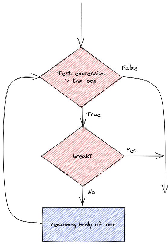
Sometimes it is useful to control the statements in a loop with a bit more precision. You may want to skip over code and proceed directly to the next iteration, or, as demonstrated in the previous section with the break statement, it may be useful to exit the loop prematurely.
41.2.2.1 Break Statement
41.2.2.2 Next/Continue Statement
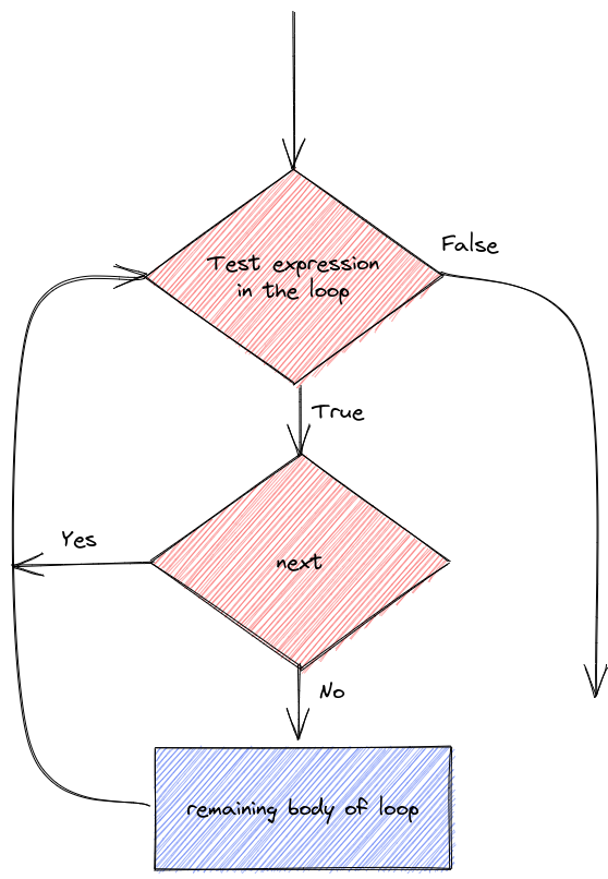
Example: Next/continue and Break statements
Let’s demonstrate the details of next/continue and break statements.
We can do different things based on whether i is evenly divisible by 3, 5, or both 3 and 5 (thus divisible by 15)
for i in range(1, 20):
  if i%15 == 0:
    print("Exiting now")
    break
  elif i%3 == 0:
    print("Divisible by 3")
    continue
    print("After the next statement") # this should never execute
  elif i%5 == 0:
    print("Divisible by 5")
  else:
    print(i)
## 1
## 2
## Divisible by 3
## 4
## Divisible by 5
## Divisible by 3
## 7
## 8
## Divisible by 3
## Divisible by 5
## 11
## Divisible by 3
## 13
## 14
## Exiting now
To be quite honest, I haven’t really ever needed to use next/continue statements when I’m programming, and I rarely use break statements. However, it’s useful to know they exist just in case you come across a problem where you could put either one to use.
41.2.3 Recursion
Under construction.
In the meantime, check out [2] (R) and [3] (Python) for decent coverage of the basic idea of recursive functions.
41.2.4 Text Encoding
I’ve left this section in because it’s a useful set of tricks, even though it does primarily deal with SAS.
Don’t know what UTF-8 is? Watch this excellent YouTube video explaining the history of file encoding!
SAS also has procs to accommodate CSV and other delimited files. PROC IMPORT may be the simplest way to do this, but of course a DATA step will work as well. We do have to tell SAS to treat the data file as a UTF-8 file (because of the japanese characters).
While writing this code, I got an error of “Invalid logical name” because originally the filename was pokemonloc. Let this be a friendly reminder that your dataset names in SAS are limited to 8 characters in SAS.
/* x "curl https://raw.githubusercontent.com/shahinrostami/pokemon_dataset/master/pokemon_gen_1_to_8.csv > ../data/pokemon_gen_1-8.csv";
only run this once to download the file... */
filename pokeloc '../data/pokemon_gen_1-8.csv' encoding="utf-8";


proc import datafile = pokeloc out=poke
  DBMS = csv; /* comma delimited file */
  GETNAMES = YES
  ;
proc print data=poke (obs=10); /* print the first 10 observations */
  run;
Alternately (because UTF-8 is finicky depending on your OS and the OS the data file was created under), you can convert the UTF-8 file to ASCII or some other safer encoding before trying to read it in.
If I fix the file in R (because I know how to fix it there… another option is to fix it manually),
library(readr)
library(dplyr)
tmp <- read_csv("https://raw.githubusercontent.com/shahinrostami/pokemon_dataset/master/pokemon_gen_1_to_8.csv")[,-1]
write_csv(tmp, "../data/pokemon_gen_1-8.csv")

tmp <- select(tmp, -japanese_name) %>%
  # iconv converts strings from UTF8 to ASCII by transliteration -
  # changing the characters to their closest A-Z equivalents.
  # mutate_all applies the function to every column
  mutate_all(iconv, from="UTF-8", to = "ASCII//TRANSLIT")

write_csv(tmp, "../data/pokemon_gen_1-8_ascii.csv", na='.')
Then, reading in the new file allows us to actually see the output.
libname classdat "sas/";
/* Create a library of class data */

filename pokeloc  "../data/pokemon_gen_1-8_ascii.csv";

proc import datafile = pokeloc out=classdat.poke
  DBMS = csv /* comma delimited file */
  replace;
  GETNAMES = YES;
  GUESSINGROWS = 1028 /* use all data for guessing the variable type */
  ;
proc print data=classdat.poke (obs=10); /* print the first 10 observations */
  run;
This trick works in so many different situations. It’s very common to read and do initial processing in one language, then do the modeling in another language, and even move to a different language for visualization. Each programming language has its strengths and weaknesses; if you know enough of each of them, you can use each tool where it is most appropriate.
41.3 Advanced Topics and Resources
- Building reproducible analytical pipelines with R by Bruno Rodrigues [4] - software engineering techniques for R programming
41.4 References
[1]
Anish Athalye, Jon Gjengset, and Jose Javier, “The missing semester of your CS education. Missing semester.” [Online]. Available: https://missing.csail.mit.edu/. [Accessed: Apr. 20, 2023]
[2]
DataMentor, “R recursion. DataMentor,” Nov. 24, 2017. [Online]. Available: https://www.datamentor.io/r-programming/recursion/. [Accessed: Jan. 10, 2023]
[3]
Parewa Labs Pvt. Ltd., “Python recursion. Learn python interactively,” 2020. [Online]. Available: https://www.programiz.com/python-programming/recursion. [Accessed: Jan. 10, 2023]
[4]
B. Rodrigues, Building reproducible analytical pipelines with R, 1st ed. Leanpub, 2023 [Online]. Available: https://raps-with-r.dev/. [Accessed: May 10, 2023]